WHAT'S YOUR SINE?
Grapher plots mathematical functions
by Delmar Searls
Quick--what does the graph of SIN(X2)*COS(X+2) look like? If you,ve ever had trouble visualizing what an equation looks like, you'll appreciate Grapher; the graph-plotting program on your START disk.
The scene: It's 11:35 p.m., and you're sitting in your dorm room, poring over a trigonometry book, staring at equation after equation full of complex mathematical functions. You grasp most of it, but it's tough to visualize exactly how some of these equations would look as graphs.
Fortunately, there's a solution: You turn to your ST and type the equations into Grapher or 3-D Grapher, the Personal Pascal graphing programs on this issue's START disk.
Grapher will automatically graph each function on your monitor screen. You can choose either a rectangular or polar coordinate system, and with a rectangular coordinate system you can choose the horizontal and vertical scales independently. Grapher works in either monochrome or color, low- or medium-res, and it allows you to choose the color of the graph.
3-D Grapher only works with rectangular coordinates, not polar--but with 3-D Grapher you can plot graphs in three dimensions and rotate them any way you like. Like Grapher, 3-D Grapher lets you choose the resolution and colors.
Grapher and 3-D Grapher are great for anyone who needs to draw graphs, including teachers and (harried) students in algebra and trigonometry classes. Since you can enter the function you want graphed, it's easy to investigate what happens to the shape of a graph when you make small changes in the function.
RUNNING GRAPHER
Grapher and 3-D Grapher work in similar ways. To use either one, copy the file GRAPH.ARC or GRAPH3D.ARC to a fresh disk, along with ARCX.TTP. Run ARCX, then type the ARC's filename; your disk drives will spin, and soon you'll have a runnable version of the program you've chosen.
Let's start by exploring Grapher, the 2-D version. When you run GRAPHER.PRG, you'll first choose a text interface or a GEM-based interface. The text interface accepts input from the keyboard only; it uses default values to keep your typing to a minimum. The GEM interface makes use of dialog boxes for all input, and the only keyboard entry is the function you want graphed.
ENTERING THE FUNCTION
To graph a function, first type it in as you would write it in BASIC. Table 1 contains a list of symbols and functions you can use. To see a sample graph, for SIN(X), simply press the Return key (or click on the OK button, if you are using the GEM interface).
Grapher draws graphs of single variable functions; the only variable you should use in your function is X. When entering numbers you may use either integers or fractions. As in BASIC, every arithmetic operation must be explicit. In algebra the expression 2X means "2 times X"; to use the same function in Grapher you must type 2 *X.
Table 2 shows how you can generate the graphs of many other common functions using the ones built into the program. It's just a matter of writing them in terms of the ones we have available.
The exponentiation operator is (error in original text) Normally this operator can only be used if the exponent's base is non-negative (The way Personal Pascal performs exponentiation prohibits negative bases.) However, Grapher is a little bit more sophisticated; it allows a negative base if the exponent is an integer.
Suppose you want to graph the cube root of X. The equation is Y = X ^ (1/3). Since the exponent (1/3) is not an integer, the function can only be evaluated (and the graph drawn) for positive values of X. To graph it all we divide it into two parts both drawn on the same grid: Y = X ^ (1/3) and Y = -(-X ^ (1/3)).
Table 1
|
In addition to integer or decimal numbers, the items in this table can be used in writing the function to be graphed by Grapher. A list of the priorities of the various operations is also included for your convenience. Functions: Binary operator: Binary operators: Variable: Grouping symbols: Priority from highest to lowest: Within an expression, two or more operations having the same priority are processed from left to right. |
|---|
Grapher will check your function carefully for syntax errors. If it finds one it points out the approximate location of the error; the actual error is usually connected with the value or symbol just before the error pointer. If an error does get by these checks and is caught when the function is evaluated, you'll get a "Postfix Error' message. Some functions may also cause floating point overflows or division-by-zero errors in Personal Pascal. (This won't happen often--and then it's usually with really weird functions )
DRAWING THE GRAPH
Grapher allows you to choose from three different grids: rectangular, polar or trigonometric. The rectangular grid is the normal Cartesian coordinate grid. A polar grid consists of a series of circles with lines radiating out from the center every 5 degrees. In a polar coordinate system, X represents an angle in radians and Y is a radius; a point is plotted by moving out the correct distance at the given angle. A trigonometric grid is a rectangular grid with the X-axis labeled in terms of (pie)/2, (pie), 3(pie)/2, and 2(pie); it's useful for graphing trigonometric functions.
After choosing the grid type you must choose the scale for labeling the graph. For example, if you choose a value of 2 for the X-Scale, the X-axis (to the right of the origin) will be labeled 2, 4, 6 and 8. Each label corresponds to a grid line. If you are using a rectangular grid, you can choose the horizontal and vertical scales independently. With a polar grid, the only scale is the radius scale which corresponds to the scale of the X-axis. With a trigonometric grid, the X-axis scale is fixed but you can choose the scale for the Y-axis.
Next you must pick a color for the graph. When you're graphing more than one equation, you'll probably want to use a different color for each function.
Finally, you must choose how the grid is to be drawn. One choice is to clear the screen, draw the grid, and then draw the graph. Another is to clear the screen but not draw any grid--the graph is simply drawn on the clear screen.
| ||||||||||||||||||||||
(Some polar equations generate pretty patterns that are better seen without the grid--try Y=SIN(121*X).) The third option is to draw the new graph on top of the previously drawn graph. This is useful when you want to show the graphs of two or more functions on the same display.
After you've entered your function and chosen the graph options, the program will automatically graph your function.
For a rectangular or trigonometric grid, the graph is drawn from left to right. After it's finished plotting, the display will remain until you press the Return key or click the left mouse button. Then the display will be saved into a buffer, and you can choose new graph options.
A polar graph has no predetermined stopping point, since the angle keeps increasing indefinitely. You can stop graphing at any time by pressing the Return key (the left mouse key will not work here). The display will remain on the screen until you press [Return] a second time or click the left mouse button.
If you enter "Q" (or click on the QUIT button) for the graph option, you will return to the function input section. This allows you to change the function and draw a different graph. To quit the program, type the letter "Q" or click on the QUIT button in response to the function prompt, and you will return to the Desktop.
3-D GRAPHER
After writing Grapher, I became interested in the problem of doing the same thing for functions with two variables. These graphs are three-dimensional, with the value of the z-coordinate dependent on the x- and y-coordinates.
The result was 3-D Grapher. Like Grapher, it lets you choose your own colors and adjust the coordinate axes. With 3-D Grapher you can also choose the viewpoint, as well as draw the graph with hidden lines.
USING THE PROGRAM
When you run 3DGRAPH.PRG, you'll find seven options on the main menu: Color, Grid, Function, View, Draw, Help and Quit. Click on the Help button to see the instructions for using the program. There are seven help screens and you can move backward and forward through them as necessary.
Watch out for one thing: When adjusting the display colors, it is possible to set the background and text colors to the same color. If this should happen you will not be able to see the mouse arrow on the color selection screen! Fortunately, there's an easy remedy--just press the Escape key to restore the default colors and leave the Color option.
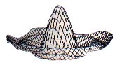
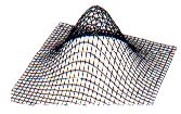 |
| Figure 1. One way of drawing graphs of three-dimensional functions. The graph is thought of as a wire-mesh. You can see right through it. |
You'll find that the most time-consuming aspect of 3-D Grapher is the calculation of the z-coordinates. With 16 grid lines per positive axis (the default) there are a total of 33 grid lines crossing each axis and 1089 points determined by the grid. The calculation for each of these points involves a number of floating point operations and function calls. In addition, the program has to evaluate the expression you entered at the keyboard, which takes more time.
The second most time-consuming aspect is the transformation of the point coordinates based on the view parameters. A new transformation is required every time you change the view-point, change the perspective option, or change the screen scale.
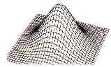 |
| Figure 2. In many cases the graph is thought of as a solid surface. In that case, nearer portions of the graph may hide portions farther away. |
For both the coordinate and transformation calculations the execution time is roughly proportional to the square of the number of grid lines. Consequently, I suggest that you stick with the default values (16 for each positive axis) until you're satisfied with the appearance of the graph.
If you increase the number of grid lines, you must also adjust the grid scale if you want the graph to have the same general appearance. Suppose the grid scale is 0.15 with the default number of grid lines. If you multiply the number of grid lines by 1.5 (up to 24 per positive axis) you must divide the grid scale by the same factor. That is, the grid scale would need to be changed to 0.10 (0.15/1.5 = 0.10). In both cases, then, the coordinate values would range from -2.4 to 2.4; by steps of 0.15 in the first case and by steps of 0.10 in the second.
In choosing colors, I've found that graphs on a black background (color intensities: 000) look really nice. I often use blue (007) for the top and red (700) for the bottom of the graph.
Figures 5 through 9 illustrate what the program can do. It takes a little bit of playing around to get a graph to look nice. In particular, a change in the grid scale can make a tremendous difference in how a 3-D graph looks. Such changes increase or decrease how much of the function will be displayed.
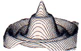
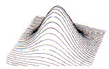 |
| Figure 3. Sometimes the graphs are drawn with only one set of grid lines. |
HOW THE PROGRAMS WORK
Grapher and 3-D Grapher face a common difficulty: evaluating the mathematical formula that you type in. The problem is that certain types of computations have a higher priority than others. For example, to evaluate the expression 3 + 2 * 4 the multiplication should be done first (2 * 4 = 8), followed by the addition ( 3 + 8 = 11 ). If we want to do the addition first, we put it inside parentheses (3 + 2) * 4
Because of different priority levels, it is fairly difficult to write a routine that directly evaluates mathematical expressions in the form we usually write them. (This form is called infix notation because the arithmetic operators come in between the corresponding operands.) Most compilers (and my program) first convert the infix expression into a form more convenient for computation. This form is called postfix notation.
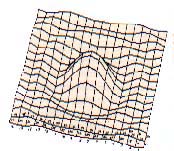 |
| Figure 4. The hidden line algorithm used in the program is based on the fact that the graph is drawn from front to back. The exact order in which the line segments were drawn on this graph are indicated by the numbers next to each segment. Enough segments are numbered to indicate the drawing order. |
In postfix notation, an arithmetic operator follows its operands. For example, the infix notation to add 2 and 3 is "2 + 3". In postfix notation it would be written "2 3 +"; the plus sign means "add the last two numbers." The big advantage to postfix notation is that the computations are performed as they are encountered. You don't need to worry about priorities, so parentheses aren't necessary.
After you've typed in the equation for your function, the infix expression you've typed is converted into a postfix expression by the procedure Convert. As the graph is drawn, the value of the postfix expression for different values of X is returned by the function Evaluate. Understanding how each of these procedures work depends on understanding a data structure called a stack.
A stack is a temporary buffer for holding data, and it works something like a stack of dishes: you only add a dish by putting it on top of the stack, and only remove it by taking a dish off the top. As a result, the last dish added to the stack is the first one removed. A data stack works the same way. Values are always added to the "top" of the stack, and the only value that can be removed is the topmost one. Because the last number you added to the stack is the first one you can remove, a stack is often described as a LIFO, or last-in-first-out, structure.
To see exactly how these programs use a stack to interpret and execute an infix expression, let's look at two of the procedures in Grapher (the 2-D version): Convert and Evaluate.
CONVERT
 |
| Figure 5. This is the default graph. If you click on the Draw option when you first get to the main menu, this is what you'll get. |
The Convert procedure changes an infix expression to postfix. It uses a data stack for temporary storage of the operators. (In this case "operators" means mathematical functions as well as the ordinary arithmetic operators.) The data stack is initialized by pushing a null element onto it, which makes it easier to detect errors in the postfix expression.
The processing algorithm scans the expression from left to right. Whenever a numeral ('0'-'9') or a decimal point is encountered, the program continues scanning until it reaches a non-numeric character. The string is then converted into its numeric form, and appended to the postfix expression.
When an alphabetical character is encountered, the program assumes it is either a function or the variable X. If it's an X, it's appended to the postfix expression. If not, the program continues to get alphabetical characters to check the spelling. The only other valid characters are arithmetic operators and left and right parentheses. Invalid characters will cause a syntax error message to be printed with an arrow pointing to the approximate location of the error.
When an operator is encountered, the program compares the operators priority with whatever is on top of the stack. Operators on the stack with a priority greater than or equal to the current operator are pulled from the stack and appended to the postfix expression. The current operator is then pushed onto the stack. Notice that if the current operator's priority is greater than that of the topmost operator, it is placed on the stack immediately.
 |
| Figure 6. Z = (Y*SIN(X) +X* SIN (Y)) *4; grid scale + 0.50; default number of grid lines. |
When a left parenthesis is encountered, it is pushed onto the stack. When a right parenthesis is encountered, operators are pulled from the stack (one at a time) and appended to the postfix expression until the corresponding left parenthesis is on top of the stack. Both parentheses are then discarded.
This algorithm is repeated up to the end of the infix expression. When the last character has been processed, the operators left on the stack are pulled from the stack one at a time and appended to the postfix expression. Finally, the null element is pulled from the stack, leaving it empty. Throughout this process, the routine must watch out for errors; for example if the algorithm is processing a right parenthesis there had better be a matching left one.
Here is the routine restated in pseudo code. PUSH places an item on top of the stack, PULL removes the top element, and "TOS" means the operator on the top of the stack.
PUSH(NULL)
 WHILE THERE ARE MORE TOKENS
  SCAN FOR NEXT TOKEN
  CASE TOKEN OF
   OPERAND: APPEND TOKEN TO POSTFIX

   "("    : PUSH(TOKEN)

   ")"    : WHILE TOS <> "("
            DO

             APPEND TOS TO
             POSTFIX
             PULL(TOS)
            ENDWHILE
            PULL(TOS)

   OPERATOR: WHILE PRIORITY
             (TOKEN) <=
             PRIORITY(TOS) DO
              APPEND TOS TO
              POSTFIX
              PULL(TOS)
             ENDWHILE
             PUSH(TOKEN)

  ENDCASE
ENDWHILE
WHILE TOS <> NULL DO
  APPEND TOS TO POSTFIX
  PULL(TOS)
ENDWHILE
PULL(TOS)
Let's work through an example: the infix expression 1 + SIN (3*4 + 2).
Infix Expression Postfix Expression Stack
1 + SIN(3*4 + 2) NULL
First, the "1" is appended to the postfix expression.
+ SIN(3*1 + 2) 1 NULL
The next character is "+" which goes on the stack.
SIN(3*4 + 2) 1 NULL +
The next item is "SIN" which has higher priority than "+" so it's added to the stack.
(3*4 + 2) 1 NULL + SIN
The next item is "(" and it is pushed onto the stack.
3*4 + 2) 1 NULL + SIN (
"3" is appended to the postfix expression.
*4 + 2) 1 3 NULL + SIN (
The "*" goes onto the stack since "(" has low priority.
4 + 2) 1 3 NULL + SIN ( *
The "4" is appended to the postfix expression.
+2) 1 3 4 NULL + SIN ( *
The next item is "+". Since "*" has higher priority than "+" it is appended to the postfix expression and pulled from the stack. The "+" is then pushed on the stack.
+ 2)                 1 3 4 *                          NULL + SIN (
2)                   1 3 4 *                          NULL + SIN ( +
'2" is appended to the postfix expression.
) 1 3 4 * 2 NULL+SIN(+
")" causes the top "+" to be appended to the postfix expression, then the parentheses are both discarded.
)                    1 3 4 * 2 +                      NULL + SIN (
                     1 3 4 * 2 +                      NULL + SIN
Since there are no more new characters, SIN and + are appended to the postfix expression.
                     1 3 4 * 2 + SIN                  NULL +
                     1 3 4 * 2 + SIN                  + NULL
Finally, NULL is pulled from the stack. The resulting postfix expression, 1 3 4 * 2 + SIN +, can then be evaluated with the procedure Evaluate.
EVALUATE
The Evaluate procedure takes a postfix expression and evaluates it from left to right, performing the necessary arithmetic operations as it goes. Unlike Convert, which uses a stack only for operators, Evaluate uses the stack only for values. As numbers are encountered they are placed on the stack. When an operator is encountered, the top one or two (depending on the operator) numbers come off the stack for the operation, and the result is returned to the stack.
For example, the postfix expression we just generated with Convert, 1 3 4 * 2 + SIN +, is evaluated as follows.
| STACK | |
| ---------- | |
| Push 1 onto the stack | 1 |
| Push 3 onto the stack | 1 3 |
| Push 4 onto the stack | 1 3 4 |
| Remove top two, multiply, and | |
| push result onto the stack | 1 12 |
| Push 2 onto the stack | 1 12 2 |
| Remove top two, add, and push | |
| result onto the stack | 1 14 |
| Remove top value find Sine and | |
| push result onto the stack | 1 0.24 |
| Remove top two, add, and push | |
| result onto the stack | 1.24 |
 |
| Figure 7. Z + 1.25* (COS(D)+COS(2*D) *2 +COS(6*D)/4); grid scale = 0.10; 32 grid lines per positive axis. The "Lines both ways" feature was turned off in the View option. |
The single value remaining on the stack is the final value of the postfix expression. If at any time there are not enough values on the stack to perform an operation, or if there's more than one value left at the end, then a postfix error occurs. This is caused by an error in the original infix expression.
When the postfix expression is evaluated the program checks for illegal arithmetic operations, such as division by zero. If this should occur, a Boolean "Undefined" is set to TRUE. The program then continues with the next value of X.
It's easy to see that evaluating the postfix expression is much more straightforward than working with an infix expression. If you're writing a program that needs to decipher arithmetic expressions, procedures like Convert and Evaluate are useful to have.
3-D COMPLICATIONS
3-D Grapher has special problems that arise because of the hidden-line and perspective features. Perspective is the easier problem; let's look at that first.
We're all familiar with perspective: If two lines are the same length but different distances away, the nearer one appears to be longer than the farther one. If this property is missing, a 3-D graph somehow just doesn't look quite right.
3-D Grapher includes a "Perspective" feature you can turn on (the default condition) or off from the View menu. The perspective transformation simply moves points that are logically behind the screen a little closer to the origin and points in front of the screen a little farther away. The distance is proportional to how far the point is behind or in front of the screen.
On rare occasions (with vertical or nearly vertical line segments) this feature can fool the hidden-line logic because the orientation of the line is altered by the perspective transformation. Changing the view angle slightly or turning off the perspective feature will correct the problem.
But what about that hidden-line logic? How does it work?
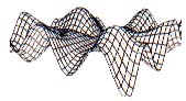
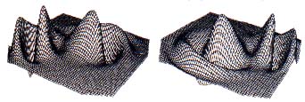 |
| Figure 8 (A and B). Z =2*(2 ^ (-((X-.5) ^ 2+(Y-1) ^ 2))-2.5 ^ (-((X+2) ^ 2+ (Y+1) ^ 2)))*COS(R); grid scale = 0.10; 32 grid lines per positive axis. This function basically superimposes two hills (the exponential functions) on a cosine curve symmetric about the origin. Two views are shown. |
The most common way of drawing 3-D graphs is to plot sections along lines of constant x and or lines of constant y. The graphs can be thought of in two different ways. One approach is to think of the graph as a wire mesh where you can see through the "surface" defined by the function (see Figure 1). The second approach is to consider the graph as a solid object (Figures 2 and 3). In that case, parts of the graph closer to the viewer can hide other portions of the graph.
There are several ways of preventing these hidden lines from being shown. The method 3-D Grapher uses is fairly old but quite effective. The key is the order in which the lines are drawn: They must be drawn starting with the closest line and working backwards to the rearmost line.
HIDING FROM FRONT TO BACK
But it's a little more complicated. Each line is drawn as a series of line segments. In most cases, one of the two sets of lines--either the constant-x lines or the constant-y lines--will be more nearly parallel to the screen (see Figure 4). Let's suppose that the lines of constant y are more nearly parallel. In addition, one end of these more nearly parallel lines will usually be closer to the viewer than the other. Let's suppose the positive end of the line is closer.
The first (that is, closest) line of constant y is drawn from right to left (positive to negative). Next, the first segment of each line of constant x is drawn, again from right to left. Then the second line of constant y is drawn right to left, then the second segment of each line of constant x, and so on. Each succeeding segment in a given line is farther from the viewer than the previous one.
The program uses an array to store the highest and lowest points plotted in each column of pixels. A point whose y-coordinate is less than (or equal to) the minimum value for the corresponding x-coordinate would be visible since it lies below the graph (or the point has already been plotted). Similarly, a point whose y-coordinate is greater than or equal to the maximum value is visible since it lies above the graph. Other points (with y-coordinates between the maximum and minimum values) would be hidden by a solid surface and thus are not shown.
To make sure that the first point tested will automatically be visible, the array of maximum values is initialized at -32767, so the first y-coordinate will always be greater than the current maximum. For similar reasons, the array of minimum values is initialized at 32767. While the screen x-coordinates range from 0 to 639 at most, the arrays extend from -640 to 1280. In effect, the program is drawing the graph on a virtual screen that is three times wider than the physical screen and hundreds of times higher.
(On the ST's screen there's a complication to all this. While a graph's y-coordinates increase from the bottom of the screen to the top, the actual screen coordinates are the opposite: The topmost row has a y-coordinate of zero and the coordinates increase as you go down. Thus in the program, if a point has a y-coordinate less than or equal to the current minimum, that point is above the graph.)
Before drawing a line segment, the program checks the visibility of the two endpoints. If both endpoints are visible, the program assumes that the entire line segment is visible and it is drawn. If both endpoints are hidden, the entire line segment is considered to be hidden and nothing is drawn. If only one endpoint is visible, the program moves along the line segment plotting the visible portions. As the graph is drawn, the minimum and maximum arrays are updated. Since the graph is drawn from front to back, regardless of the viewing angle you choose the program can figure out how to draw the graph properly.
The hidden lines feature is active when you start the program; you can turn it off from the View menu. If you turn it off, the graph is drawn much faster, but of course it may be a little harder to visualize.
THE SLOW OPTION
It may have occurred to you that even if both endpoints of a line segment are visible, that doesn't necessarily mean the entire segment will be visible. That's a good point, although it's quite rare for only the middle portion of a line segment to be hidden. If it should occur with an equation you're trying to graph, try increasing the number of grid lines. That makes the line segments shorter and decreases the chances of this kind of error.
3-D Grapher also offers a second solution. Normally the program runs with the "Fast plot" option turned on (the default). If you turn this feature off from the View menu, the program will no longer make assumptions based on endpoints. Instead, it will plot only the visible points in each line segment on a point-by-point basis. This approximately doubles the drawing time, though it's still quit fast.
THE PRACTICAL ST
With its graphics power, processing speed and low price, the ST is the perfect computer for students, or anyone who wants a practical tool for exploring higher math. Many people complain that there isn't more practical applications software for the ST. I hope Grapher and 3-D Grapher fill a need, and become a useful tool for students, mathematicians, and anyone who's simply curious about what an equation looks like.
Delmar Searls hopes to use the StereoTek glasses to produce 3-D Grapher in true stereo vision.