OMNI LIFE
by Tom Hudson
Tom Hudson is a freelance programmer who has to his credit such classic ST software packages as DEGAS and DEGAS Elite, as well as the CAD -3D family of graphic tools.
One of the oldest computer games in existence today is a simple simulation called Life. Originated by John Conway in 1968, the game is often referred to as "Conway's Life." The game is a simulation of the life cycle of single-celled organisms, which is determined by simple rules, or parameters. The term "game" as used here doesn't mean it's a cellular-level shoot-em-up or adventure, but rather an exercise in logic. I prefer to think of Life as a simulation, but I'll leave the hair-splitting to you.
Due to the large size of this program, it is available only on this month's disk version or in the databases of the DELPHI ST-Log users' group.
The Facts of Life
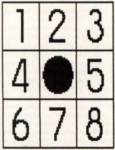
The original Life is played on a two-dimensional grid, which serves as a sort of binary petri dish where we can watch our cells grow, multiply and die. Each location on the grid has eight neighboring grid locations, as shown in Figure 1.
In the standard Life, a cell is born if there are exactly three live cells in the grid locations surrounding it. A live cell will die if there are fewer than two or more than three cells surrounding it. The analogy generally used here is that a cell dies of starvation if there are fewer than two neighbors, and dies of overcrowding if are more than three neighbors.
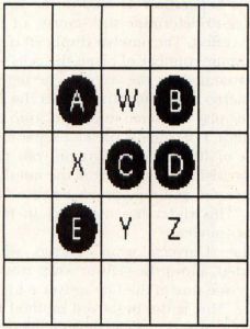
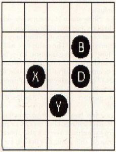
With this in mind, look at Figure 2. There are five cells alive in this illustration, labeled A through E, and four unoccupied grid locations, labeled W through Z. Let's look at this setup and find out what will happen next.
Cell A only has one neighbor, cell C. It will die of starvation and will not be present in the next generation. Cell B has two neighbors, C and D, and will live to the next generation. Cell C had four neighbors, A, B, D and E. It will die of overcrowding. Cell D has two neighbors, B and C, so it will live. Cell E only has one neighbor, C, so it will die.
Now that we've determined which cells will live to the next generation, let's look at the empty grid locations W, X, Y and Z. Location W has four neighbors, A, B, C and D. Since exactly three live neighboring cells are required for a birth, no cell will be born there. Location X has three neighbors, A, C and E, and a cell will be born there. Likewise, location Y has three neighboring cells, C, D and E, and a cell will be born there. Location Z has only two neighboring cells, C and D. No cell will be born there.
After the status of all the grid locations have been determined, a new cell grid is plotted according to the results. Figure 3 shows the cell grid for the generation following the example in Figure 2. The cells are labeled according to the letters used in Figure 2.
This simple procedure is carried out for each location on the grid, and continues until there are no live cells or the user stops the process.
The original Life uses the parameters previously stated for the simulation of cellular growth: For a live cell to survive, a minimum of two neighboring cells and a maximum of three neighboring cells is required. For a cell to be born a minimum of three neighboring cells and a maximum of three neighboring cells is required. In a kind of shorthand notation, this would be known as Life 2333.
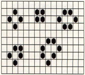
Life 2333 has a great variety of "life-forms," which can be stable or cyclical. A stable lifeform is one which retains its form for an infinite period of time, without moving, as long as it is not affected by other cell "colonies." Figure 4 shows some of the stable lifeforms.
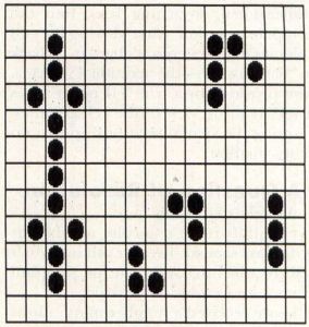
Cyclic life forms are those which change shape from one generation to another, eventually returning to their original form. Perhaps the most interesting of these forms is the "glider," a cell group which goes through a four-generation sequence, and moves one grid diagonally in the process. As a result, it appears to "swim" across the screen like a tadpole, complete with a wiggling tail-like structure. Figure 5 shows some of the more common cyclic lifeforms. The glider is in the upper right corner.
There is nothing preventing us from running Life simulations with other parameters. Life 2333 is simply the classic standard version, and is a good starting point for new "Lifers." Some parameter sets may be more pro-life, with rapid overpopulation; others anti-life, with cells meeting their end quickly.
The Third Dimension
The original Life, as mentioned above, operates strictly in two dimensions, resulting in a simple plane of cells. Recently, in his Scientific American "Computer Recreations" column, A.K. Dewdney addressed the possibility of creating Life programs which operate in three dimensions, giving incredible possibilities for new lifeforms. Such a 3-D Life program requires a high-speed processor for reasonable speed in processing the cell matrix; it also requires a graphic display which can show a reasonable approximation of the 3-D group of cells. Fortunately for us, the ST computers have both.
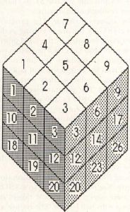
Three-dimensional Life is an incredible extension of standard 2-D Life. It can display many of the same kinds of lifeforms as 2-D Life, but modified somewhat in order to operate in three dimensions. The primary difference between 2-D and 3-D Life is that in the 3-D version each cell has 26 neighboring cells: Nine in the plane above, nine in the plane below, and eight surrounding the cell in its plane. This forms a three cell by three cell cube with the center cell of the cube being analyzed. The layout of the cube is shown in Figure 6. I won't go into laborious detail here with an analysis of the Life process in three dimensions; it is exactly like the 2-D process except that there are 26 neighboring cells to check.
As you have probably already guessed, the parameters for 3-D Life are different from those of 2-D Life. Since there can be up to 26 neighbors rather than eight, the parameter count can range accordingly. According to Dewdney, the parameter set for 3-D Life which shows the most promise is 4555 (four-five neighbors to stay alive, and exactly five neighbors to be born). A secondary parameter set he mentions is 5766, which apparently mimics the 2-D Life 2333 more closely.
Introducing OmniLife
Spurred by the Scientific American article, I sat down and wrote OmniLife, a program which will run both 2-D and 3-D Life simulations. The program allows you to set all sorts of Life parameter sets in order to test different rules for lifeform generation. It also includes a cell editor screen for both 2-D and 3-D start-up cell groups, as well as random "primordial soup" cell groups, for the anarchists out there.
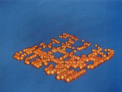
But perhaps the most exciting feature of OmniLife is the ability to show cell colonies in true stereo by using the LC Technologies StereoTek glasses. With these optional glasses, you can run 2-D or 3-D Life simulations which are actually three-dimensional, stretching back into the computer monitor. After viewing the cell colonies in true stereo, it's hard to go back to "flat" displays—the additional information provided by a true 3-D image gives a very realistic view of the cell colonies, showing the spatial relationship like no other method.
A Question of Resolution
A slight digression here.
OmniLife requires a color monitor, as it displays shaded, 16-color cell images. It also requires that you run the program from a low-resolution desktop.
I have received a number of questions from ST users as to why some programmers seem to be "lazy" and force you to start a program in certain resolution, when it's possible for the ST to change screen resolutions at any time.
The answer is simple. The programmers aren't lazy, but are operating under a restriction imposed by the GEM graphics environment. Let's say I needed to run a program in medium resolution, but started it in low resolution and switched to medium resolution after starting up the program. The programmer can now do things on a 640 by 200 pixel screen, but there will be problems. As far as GEM is concerned, it's still running in low resolution. The mouse arrow will only go halfway across the screen because GEM thinks the screen is only 320 pixels wide. Dialog boxes and drop-down menus won't be drawn correctly, either.
Going from medium to low resolution is worse. You're now working in a 320 by 200 pixel screen, while GEM thinks it's working with 640 by 200. The mouse arrow will go from the left side of the screen to the right, then wrap back around again to the left side and to the right before it stops! This is because the mouse handler is operating with a 640-pixel wide screen, which is twice as wide as the low-resolution 320-pixel screen.
If you have a dialog box which uses more than four colors in this case, only the first four colors will be displayed, because GEM thinks you're in medium resolution, with a four-color limit.
There are ways around all these problems, but working around them means abandoning the GEM user interface, with its common ground for all programs written using it. Programmers aren't lazy when they follow the GEM programming guidelines and force you to start a program in a given resolution. They're merely following the proper procedure which will allow their programs to run correctly when a new ST computer or set of ROMs is introduced. It's a limitation and an annoyance sometimes, but don't blame the programmers.
Back to Life
The program OMNILIFE.PRG on your ST-Log disk is the OmniLife program. When you run this program, be sure your computer is running in low-resolution. OmniLife uses the low-resolution screen for a colorful display and since it uses the mouse cursor for cell editing, it must be run in low resolution for proper mouse limits to be set.
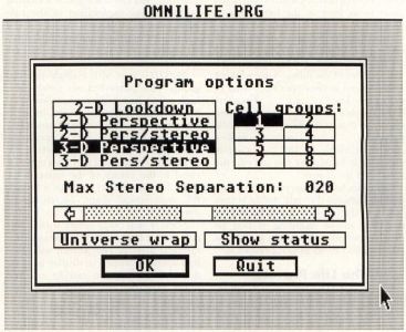
When you start the program, the first thing you will see is the program credits display. Click on OK and the program options dialog will appear, as shown in Figure 7.
The program options dialog allows you to set the main operating mode of the program (2-D or 3-D, monoscopic or stereoscopic), as well as the number of groups of cells to randomly create if the random setup mode is used and the stereo separation amount if the stereo mode is used.
There are five operating modes. These are:
2-D Lookdown: The classic Life mode, looking down on a 32×32 plane of cells from above.
2-D Perspective: A view of the 2-D Life plane in perspective from above and to one side. This mode is sometimes referred to as 2 1/2-D.
2-D Perspective/Stereo The 2-D Perspective mode, with the added effect of stereo vision, requires the LC Technologies StereoTek glasses. If you are running OmniLife without the glasses and the cell display seems to flicker with a double-image, you have accidentally selected the stereo mode.
3-D Perspective: The non-stereo 3-D Life mode. This generates a 2 1/2-D image of the cell matrix in perspective from above and to one side. This is the default mode.
3-D Perspective/Stereo: The 3-D perspective mode with stereo vision, requires the LC Technologies StereoTek glasses.
If you are going to have the program randomly generate several groups of cells rather than editing the starting status of the cells manually, you can select the number of cell groups to randomize, from one to eight. These groups will be spaced randomly throughout the 32×32 cell grid (2-D) or the 32x32x32 cell matrix (3-D), providing a sort of "primordial soup" from which lifeforms may or may not grow.
The horizontal slider, labeled "Max Stereo Separation" is used in the stereo modes to determine the severity of the stereo effect. The number displayed is the maximum number of pixels the cells will be separated on the screen. The higher the stereo separation, the further the 3-D cell display will seem to go back into the monitor. I personally prefer a separation value of 40, but depending on your particular vision, distance from the monitor, and so on, you may prefer another setting. This slider has no effect in non-stereo modes.
The "Universe wrap" button, when selected, allows the cells to wrap-around from one side of the Life universe to the other. This is the preferred method for most people, as it allows moving lifeforms like gliders to roam the universe without stopping at the edges. If the Wraparound option is not selected, objects will stop when they hit the sides of the 2-D grid or 3-D matrix.
The "Show status" button, when selected, displays various information at the bottom of the screen in both non-stereo and stereo modés. The status line will tell you how many generations have been processed (up to 32,767) and the number of cells currently alive. In 2-D mode, with its 32×32 cell grid, the maximum number of live cells is 1,024. In 3-D mode, the maximum number of cells is 32x32x32, or 32,768.
Once you have set the parameters to the desired settings, click on OK or press Return to continue. You can also abort the program at this point by clicking on the "Quit" button, but with a program this fun, who wants to quit?
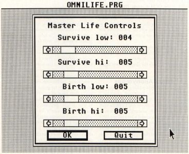
The next dialog you will see (assuming you didn't quit on the last dialog) is the Master Life Controls dialog, shown in Figure 8. This dialog has four sliders in it, which set the Life parameters we discussed earlier. When you initially start the program, the default parameters will be 2333 for 2-D and 4555 for 3-D Life. You can change each of the controls to any number of cells from one to the maximum number of neighbors (eight in 2-D, 26 in 3-D).
The first two sliders control the minimum and maximum number of neighbors which allow a live cell to survive. The first slider, "Survive low" must be less than or equal to the second slider, "Survive high." If a live cell has fewer than "Survive low" neighbors or more than "Survive high" neighbors, it will die.
The second two sliders control the minimum and maximum number of neighbors which allow a dead cell to be born. Once again, the first slider of these two, "Birth low," must be less than or equal to the second, "Birth high." If a dead cell has at least "Birth low" neighbors and not more than "Birth high" neighbors, it will come to life.
When you have set the life parameter sliders, click on OK to continue. The program will check the slider controls to make sure you haven't entered improper values in your sliders, and will warn you if you have. Once again, if you want to quit at this point, you may do so via the "Quit" button. But why quit when there's so much fun ahead? Let's press on.
Pressing On
Since you're still reading, I'll assume you pressed OK. At this point, a small dialog will appear and ask you if you want to use a random initial cell setup or a user-defined setup. Clicking on "Random" will start the Life simulation using the number of cell groups specified in the Program Options dialog (Figure 7). The program will generate some cells in a random pattern and start the simulation.
If you want to try creating your own lifeforms or patterns for the initial setup, you can do so with the OmniLife cell editor, which is used if you click on the "User" button. The editor screen is very simple. When the editor is in use, the screen will clear and the mouse arrow cursor will appear. The cell box is in the center of the screen. Moving the mouse into the box and pressing the left button will create a cell in that location. You can "draw" a cell pattern quickly by holding the left mouse button down and moving the mouse. Clicking on a cell that is already ready there will put the editor into erase mode, erasing that cell and all others you point to as long as the left button is pressed.
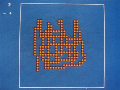
In 3-D mode, the editor allows you to edit a "slice" of the 3-D Life matrix. There are 32 slices, numbered from zero to 31. The number of the slice you are working with is shown in the upper left corner of the screen. The "+" and "-" characters below the slice number are controls allowing you to change the slice number. Clicking on the "+" control increases the slice number; clicking on the "-" control decreases it. In this way, you can edit the entire 3-D life matrix.
Once you have set up your initial Life pattern, pressing the right mouse button will begin the Life simulation. Because of the GEM mouse handling, it may be necessary to press the mouse button for a half-second or so to get a response.
The Life Process
Once you start up the Life simulation, the computer will process the cells until none are left alive or you stop the simulation. If all the cells die, a "NO LIFE" message will appear and the simulation will stop. The following keypresses are used by the program during the simulation mode:
Undo: Quits the program, taking you back to the GEM desktop. True Life fans will never use this key.
Help: Allows you to restart another simulation using the same parameters as the last one. You will be prompted for either a random or user-defined starting configuration.
F10: Returns you to the Program Options dialog to change the main operating mode of the program.
Space bar. Pauses the display. Press again to resume.
Lifers Anonymous
Life is a strangely addicting simulation. The first assembly language program I ever wrote for a microcomputer was a Life program, written on my old Compucolor II system in 8080 assembly language. It was crude, but I learned a lot and got kind of hooked on Life. When I saw the Scientific American article on 3-D Life, I couldn't resist. The added dimension of stereo vision was something I couldn't pass up, and if you try it, you'll see how important stereo vision can be on computers for giving realistic depth perception.
Following are some interesting parameter sets I have found by playing with OmniLife into the wee hours of the morning. You can use them as a starting point in your exploration of the Life phenomenon. I have a feeling you'll spend a lot of time watching lifelike patterns of cells crawl over the face of your monitor.
3-D/3311—Start with a single random group. This parameter set produces a high-population generation, followed by a large-scale reduction caused by overcrowding, then another high-population generation, and so on. Lots of interesting cubic patterns, very nice in stereo.
3-D/2344—Start with a 2×2-cell cube, located at the center of the universe, in slices 15 and 16. This will start a beautiful, symmetrical shape. Incredible in stereo.
2-D/3311 and 3322—Start with a few cells at the center of the universe in a symmetrical pattern. The pattern will grow into a kaleidoscope-like display in lookdown mode that you can let run for hours. Very nice, and it apparently does not repeat.
2-D/1233 and 1244—Use several random groups. These parameters usually cause a quick general thinning of the population, leaving many groups of one, two or three cells in stable configurations. It also leaves some interesting cyclic lifeforms.
The Details
The OmniLife source code has been provided on the STLog disk for programmers to examine and modify. It is in two parts; a C source file and an assembly language source file, and an additional file for the stereo glasses driver software.
Whenever I write a program which requires high-performance operation, I like to set it up so that the parts which require a great deal of speed are written in assembly language. Compilers are notorious for producing inefficient code, and hand-coded assembly language results in a program that runs as quickly as possible.
The problem with assembly language is that it can become cumbersome in some cases, usually in those routines which won't benefit much from assembly language speed, such as dialog handling, GEM calls, and so on. For this reason, I use C for the user-interface details of a program. It is easy and quick to code, and since it is dealing with user input in most cases, it operates fast enough for most applications.
As you can guess, the OmniLife C source module takes care of all the user interface details, such as dialogs and the cell editor. If you look at the C source file, you will see that it is pretty straightforward.
The first third of the C source file deals with the processing of the dialog boxes and their associated slider controls. The sliders are simple constructs, built out of four objects with the GEM Resource Construction Set (RCS). All the objects in a slider are TOUCHEXIT objects, and when the user clicks the mouse on one of them, they are processed by the do__hslider() function. An in-depth discussion of the operation of the slider routines can be found in the article "Handy-Dandy Slider Subroutines," in STLog 10.
The next portion of the program deals with the actual setup and operation of the Life simulation. Most of the real work is performed by the assembly language module, which contains the life2d() and life3d() functions. As a result, this code is very simple to understand.
You will notice the use of the stereo__switch() function at several points in the C source. This is the function which turns the stereo glasses on or off, and is found in the STEREO.S assembly source file. A value of one in the first parameter of this function turns the stereo glasses on; a value of zero turns them off. The last two parameters are the addresses of the left-eye and right-eye view bitmaps, respectively. This function is only used in stereo mode.
The remainder of the C source file is mostly miscellaneous support functions for the program, such as dialog utility functions. One important function is the editor() function, which performs the cell editing operations.
The editor() function is pretty much self-explanatory. It watches the mouse, and if the left mouse button is pressed inside the cell-editing rectangle, the routine either draws or erases cells. The cell array used to store the cell-status values is the three-dimensional character array, cell[][][]. A one in any array location indicates a live cell; a zero indicates no cell. Cells are drawn by the quikblit() function, a custom bit-block drawing function which operates much faster than the ST's built-in routines. Since several thousand cells are plotted on some 3-D Life simulations, speed was important here. The Atari blitter chip may be faster than this software blit. Cells are erased via the vr__recfl() function.
Assembly Source
The assembly source code is rather lengthy, but contains only a few major routines. The main Life simulation functions for two-dimensional and three-dimensional Life, life2d and life3d are respectively. These are coded for speed rather than compactness, a necessity when processing the 32,768 individual cells in the 3-D version. Tests are done to see whether or not the cell being tested lies on the edge of the matrix. If it is on one or more edges and the wrap-around mode is enabled, the cell is handled by a special section of code which handles the matrix wrap-around.
As you can see in the source code, the cells are addressed by using the A5 address register as a pointer into the cell array, with the A4 register containing a pointer into a second cell array, which contains the cell status for the next generation. At the end of the processing of the current generation, the next generation cell array is copied back into the current generation cell array. Note that both cell arrays are byte arrays, but are word-aligned so that the copying of one array to the other can be done with long moves, which are faster than four single-byte moves.
Each cell in the matrix is checked to see how many neighbors it has. This number is compared to the master life parameters, and the new state of the cell is set in the cell2 array. At this time, if the cell is alive, the cell is plotted on the screen by the do__cell subroutine (2-D/3-D perspective) or the do__cell2 subroutine (2-D lookdown only).
The do__cell routine takes care of all the coordinate handling, perspective and stereo effects, if the stereo switch is enabled. To perform the rotation of the cells so that we look down on them from one corner, the routine rotates the coordinates 45° through a fixed-point math scheme. The scheme is a simple one I developed while writing a Battlezone program for the Atari 8-bit computers several years ago. Basically, it uses a long value to store a number with a pseudo-decimal format. The high-order word contains the whole number portion, and the low-order word contains the fraction. A value of 2.5, then, would be stored as:
(2*65536) + (.5*65536) = 163840
This can easily simulate a floating-point numbering system to a fair degree of accuracy, storing fractions down to 1/65536, or .000015.
The cell coordinates are rotated by 45° in this manner, and the resulting Z value is used to calculate a size for the sphere that is to represent the cell on the screen. There are ten sphere sizes, from zero to nine.
Using the Z value again, a simple perspective transformation is applied to the cells.
This transformation is:
ScreenX = (X/(Z + 600))/600
ScreenY = (Y/(Z + 600))/600
To get stereo effects, the stereo separation is added to the X value for the left eye and subtracted from the X value for the right eye. On non-stereo simulations, the stereo separation is set to zero in order to have no effect.
The cell location is calculated, then the quikblit subroutine is called to plot the cell.
The Quikblit Routine
During development of OmniLife, the plotting of the cell spheres seemed to take quite a bit of time, especially on stereo simulations, which obviously need twice the processing time in order to draw both the left- and right-eye views. I thought about it a little, and decided to code up a simple bit-block transfer (bitblt) routine for the ST's low-resolution mode. The fact that none of the spheres that represent the cells are greater than 16 pixels wide was a major part of my decision, since it would simplify the bitblt operation to operate on word-wide blocks of data. The cells are all designed to be 13 pixels high, even though the smaller cell images do not use the entire height.
The quikblit routine requires five parameters:
Bitmap address: The base address of the screen where the block is to be drawn.
Mask address: The address of a single-plane pixel mask for the image to be plotted. This mask is ANDed with all four destination bitplanes in order to "cut a hole" in the image where our cells can be plotted. Without this hole, the cells would show through each other.
Image address: The address of the four-plane image data.
X coordinate: The X coordinate on the screen of the center of the cell. The quikblit routine adjusts this value to the left. Seven pixels.
Y coordinate: The Y coordinate of the center of the cell. The quikblit routine adjusts this value up toward the top of the screen by five pixels.
The quikblit routine performs two operations. First, it uses the mask data to make a "hole" in the image on the screen, then it uses the image data to fill that hole. The mask data is ANDed with the screen to make the hole, and the image data is ORed with the screen to place the image.
Looking at the assembly source, you will notice several blocks of data for the cell sphere images. There are two sets of cell image data, one for the left-eye and one for the right-eye view. The spheres for the right-eye view have the yellowish highlight shifted to the left somewhat in order to simulate the difference in the highlight on a spherical object as seen by the two eyes. The images were created with DEGAS Elite and converted to DC.W data lines.
Both the mask and image data are shifted into the proper alignment with the screen by using the 32-bit data registers to hold the 16-bit mask or image data. The two halves of the shifted value are processed, first the low-order 16 bits, then after a SWAP operation (where the high-order 16 bits are moved to the low-order 16 bits) the high-order bits are transferred to the screen.
The quikblit routine is made faster by the fact that it does not do any horizontal bounds-checking. The data being transferred cannot overlap the sides of the screen, or improper images will result. The same goes for the top of the screen. The bottom of the screen is properly handled, however, since some of the cells plotted by OmniLife may run off the bottom. Cells are clipped to the proper limits there.
Life Goes On
I hope you find OmniLife to be as enjoyable as I do. It is an interesting exercise, and I often find myself mesmerized by the patterns of cells on the screen. As soon as one simulation ends, you may find yourself starting up another with a slightly different cell pattern. There are an almost infinite combination of cell patterns and parameters, so get to it!
On another note, I hope some of the techniques and routines in the program source are helpful to programmers out there. The quikblit routine may be one of the more useful ones, but those people interested in 3-D and stereo should find the 3-D and stereo transforms of the assembly code particularly illuminating.