ULTRA-GRAPH
APPLICATION ANY RESOLUTION
By Blake Arnold and Phil Mast
Due to the large size of this program, the GFA BASIC listing could not be printed in the magazine. The complete program, including a compiled version that will run without GFA BASIC, is available on this month's disk version or in the ST user's group on DELPHI. See "Database DELPHI" in this issue for further information on getting a DELPHI account.
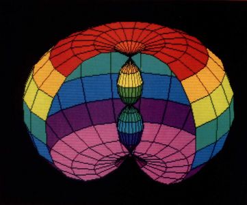
Ultra-Graph is a two- and three-dimensional graphing program. Despite the complexity usually associated with powerful graphing program, Ultra-Graph is relatively easy to use and understand, because we have gone to great lengths to make sure that complex calculations are not required to operate the program. In fact, Ultra-Graph is almost fully automated.
Ultra-Graph began as a simple three-dimensional plotting program and slowly evolved into its present state over the period of almost a year. (Okay, we did take the summer off!) As we got closer and closer to finishing it, we always found another feature that would be nice to add. Originally the program was able to graph equations only in the rectangular coordinate system, but eventually other coordinate systems were added. As it stands now Ultra-Graph is capable of graphing equations in Cartesian, polar, rectangular, spherical and cylindrical coordinate systems in any screen resolution.
The program itself is written in GFA BASIC, and the source code is relatively easy to follow so we're not going to give you a line-by-line analysis of the program. What we will do is give you a little information about the program, and a few hints the program projects a three-dimensional image on a two-dimensional screen or how the perspective effect works, that information can be found in the Abacus book Atari ST 3D Graphics.
Coordinate Systems
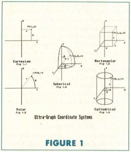
Ultra-Graph supports a total of five different coordinate systems for plotting equations. (See Figure 1). Cartesian and polar coordinate systems produce two-dimensional; rectangular, spherical and cylindrical coordinates systems are used for graphs in three-dimensional space. An almost infinite variety of shapes can be created by graphing various mathematical functions within these five coordinate systems.
The simplest of the five coordinate systems is the cartesian system (Figure 1.1). Using this system any point may be located in the x-y plane by plotting its x and y displacement (distance) along the respective axes. Plotting a series of these points provides a two-dimensional graph.
The rectangular system (Figure 1.2) is a three-dimensional adaptation of the cartesian system that is produced by rotating the x-y plane into a horizontal position and adding a z axis perpendicular (vertically) to it. A three-dimensional graph will result by measuring displacements along the x, y and z axes and plotting the associated points.
Another useful way of locating points is by using polar coordinates (Figure 13). This system locates a point in a plane by its distance (r, or radius distance) along a ray emanating from the origin at an angle (theta) measured from an initial ray. The initial ray is a horizontal line beginning at the origin pointing to the right.
As we did with the cartesian coordinate system to create the rectangular system, we can add a z axis to the polar system to create a three-dimensional system called the cylindrical system (Figure 1.4). The r-theta plane is positioned horizontally and the z axis extends vertically through the plane. The angle theta is measured horizontally from an initial ray pointing out toward you, and the distance z is measured along the z axis. The distance r is always measured perpendicularly to the z axis. This characteristic makes the cylindrical system convenient for graphs for which there is an axis of symmetry such as cylinders and cones.
The final three-dimensional system is the spherical system (Figure 1.5). It is useful for graphs that have a point of symmetry; the perfect example, as the name implies, is a sphere. When using the spherical coordinate system, all distances are measured from a single point, the origin. Points are located by an angle (theta) measured horizontally, an angle (phi) measured vertically, and its radius distance (r) from the origin.
In trying to understand the spherical coordinate system, it helps to realize that the angles of the spherical system are related to the latitude and longitude measurements of points on the earth used in navigation. The angle phi is the latitude and the angle theta is the longitude. There are differences in the points from which the angles are measured but the basic principles are the same.
How the program works
Maximum and minimum values for each argument of the function are specified by the user in the main menu. The values of the arguments are steadily incremented through the range specified and the equation is evaluated with each of these values substituted into the equation. The number of points calculated is specified by the user by the point intervals of each argument in the main menu.
The value of the function is checked each time to see if it exceeds the maximum value specified by the user; if it does these values are discarded as errors. An array is constructed of all the points, and maximum and minimum values are tracked for drawing axes and coloring. No matter what type of coordinate system is selected, the points are all converted to the rectangular system for plotting.
After computing points, a matrix is constructed for projection onto a two-dimensional plane (your monitor screen). The orientation of the plane and its distance are determined by the eye position, and the size of the graph is determined by the zoom factor. The three-dimensional points are then converted by some matrix algebra to two-dimensional screen coordinates, and the maximum and minimum values of the screen coordinates are computed for auto-centering and auto-scaling. The first point of the graph is plotted and each succeeding point has a line drawn to it to complete the graph.
Using the program
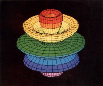
We recommend using Ultra-Graph in low or high resolution. Low resolution is preferred because of the ability to use color gradients; high resolution produces excellent definition of the graphs. The program will function normally in medium resolution, but the graphs will lack the color gradients of low resolution and the definition of high resolution.
If you have a 520 ST (that hasn't been upgraded to one megabyte of RAM), before you boot the program make sure you have no desk accessories installed and no programs in an AUTO folder on your boot disk that remain memory resident. The program doesn't leave much memory free in a 512K ST because of its point arrays and the extra screen it stores in memory, so it's possible that you won't have enough memory if you use accessories. (The program will not allow you to access them anyway; our version of a subtle hint.)
The mouse itself has a few hidden uses that should be understood before using the program. A click on the right mouse button will toggle the display between the actual plotting screen and the selection screen. (There are essentially two screens that remain in memory and alternate) Clicking on both buttons at the same time has the same effect as clicking on "Graph it!" under the "Options" drop-down menu. There is a little trick here, though; if you click on the right button before the left it will just take you to the other screen, so you'll have to press and hold the left button down and click on the right button to get the desired effect.
The drop-down menus
Although the drop-down selections aren't very complex, they do require a little explanation. Most drop-down items are straightforward, but selecting certain ones will void others or change the way they perform. Because of this we will explain each menu item, and the interrelations it has with other program options if applicable.
The File menu
NeoChrome Save: Saves a picture of the current graph (and its associated color palette) in NeoChrome format.
DEGAS Save: Saves a picture of the graph (and its associated color palette) in DEGAS format.
CAD-3D Save: Saves the graph as a CAD-3D (2.0) object that may then be loaded into CAD-3D and manipulated as a normal CAD-3D object. Valid only in three-dimensional coordinate systems. For more detailed information please refer to the "Saving CAD-3D Objects" section of this article.
Save Parameters: Saves the parameters and equation that created a graph for later recreation. Parameter files follow a special format and are not designed to be user edited.
Load Parameters: Loads a parameter file and allows the original graph to be redrawn without the user entering any information. Parameter files have a number in the extender (for example, SPHERE.PM1) that refers to the resolution that they were saved in (similar to the way DEGAS uses PI1,, PI2 and PI3 to determine picture resolution).
When a parameter file that is in the current screen resolution is loaded, the Autoscale and Autocenter features will be temporarily disabled to speed the drawing of the graph and also allow it to be viewed exactly as it was saved (i.e. with a modified center or zoom). If the parameter file's resolution information does not match the current screen resolution, Autocenter and Autoscale will be enabled, even if the graph's parameter file was saved with a modified center or zoom. This is necessary in order for the graph to appear on the screen at all.
Quit: Exits the program and returns the user to the Desktop.
The Options menu
B/W Swap: Changes the background color of the screen to white and the color that the graphs are drawn in to black. In high resolution it reverses the background color. It is intended primarily for printouts of graphs.
Gradient Changes the color palette to one of three (red, green or blue) gradually shaded palettes (low resolution only).
Rainbow: Changes the color palette to a rainbow gradient. It is perhaps the easiest palette to work with, since small details can result in large changes in the color of the graph (low resolution only).
Elevation: Changes the color palette to an elevation map palette (low resolution only).
Fill Pattern: This changes the pattern that is used to fill the polygons that three-dimensional graphs are drawn with (valid only with Hidden Lines enabled). It is selectable from empty to solid-fill. Options are shown visually. To select a fill-pattern, click on the desired pattern with the mouse.
Grid Lines: Valid only in two-dimensional coordinate systems, this option will draw numbered axes on the screen or number a side, top, or bottom of the screen if an axis is out of the screen range It will disable (until it is de-selected) the Draw-Axes option.
Hidden Lines: Valid only in three-dimensional coordinate systems, this option determines whether the graph will appear as a solid object (hidden lines enabled) or a wire-frame object.
Draw Axes: Draws the appropriate unnumbered axes superimposed on the graph. Positive axes appear as solid lines, negative axes appear as dashed lines. Note that when in a two-dimensional system, both Draw Axes and Grid Lines are initially selectable, but when one is selected, the other becomes void. (Both will become selectable again if the currently selected one is turned off). The reason is that the Grid Lines option does draw the axes, so there's no reason to have the program go back and recalculate them for the Draw Axes option. Draw Axes is also valid in 3-dimensional coordinate systems.
Auto Center: Automatically centers the graph on the screen, whether or not the entire graph appears on the screen.
Auto Scale: Automatically scales the graph to fit the screen.
Graph it!. Draws the graph from the current settings.
Demo Mode: Cycles through each of the coordinate systems and graphs one of the predefined functions for each. The only way out of the demo is to hit the Escape key after the program is finished drawing a graph. Due to what we think is a bug in the GFA Compiler, Demo Mode currently exits to bombs in the compiled program, but the runtime version performs flawlessly.
Defaults: Restores the default settings to the program.
System
Cartesian: Graphs functions in the cartesian coordinate system (two-dimensional).
Polar: Graphs functions in the polar coordinate system (two-dimensional).
Rectangular. Graphs functions in the rectangular coordinate system (three-dimensional).
Cylindrical: Graphs functions in the cylindrical coordinate system (three-dimensional).
Spherical: Graphs functions in the spherical coordinate system (three-dimensional).
Main screen options
The main screen options are a little more complex than the dropdown menu selections, but once you understand their functions, they're relatively easy to use. Most are heavily interrelated, so we will go into a little more detail with the explanations.
Function: Selecting this item allows the current function to be changed or edited. For detailed information on changing functions please refer to the "Changing Functions" section of this article.
Zoom: Changing the zoom factor moves the point of view closer (small values) or farther away (large values) from the graph. It temporarily disables the Autoscale option. (Autoscale will defeat the changed zoom if it is left enabled.)
Eye Position: These three values change the viewpoint of the graph, relative to their respective axes. Larger values increase the distance along that particular axis. It's possible to get over, under, beside or anywhere else around the graph. Extremely high values should be avoided, as should values that might be inside or on a graphed object. If the Eye x (Ex) or Eye y (Ey) positions are within the range that the graph is drawn in, the graph will be distorted severely. (This is caused by the perspective factor that is used). Eye Position values are valid only in three-dimensional coordinate systems.
Screen Center: These two values change the apparent center of the screen relative to the graph. If they are changed, the Autocenter option will be temporarily disabled.
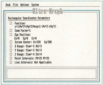
Range Values: These values change the size and relative position of the box that the graph is drawn in. Changing any of the high or low limits will terminate the graph at those points (x-hi and x-lo, etc.). For example, setting rectangular limits of X from 0 to 5, Y from 0 to 5, and Z from 0 to 5, would give you the portion (if there is a portion) of the graph in that "box." The program keeps track of the box's position and it will display an error message if no part of the graph lies within those bounds. Range values should also be kept to reasonable limits, or the perspective effect will distort the graph.
Point Intervals: The Points (Px and Py) selection will alter the number of points that the program will calculate in that particular plane Zero is not allowed, and it is recommended (in most cases) that it be kept over 20 for any detail at all.
More points produce more detail, but the calculations will take a few seconds longer. Using an excessive number of points might result in a cluttered look for some functions.
The number of points used in each direction is always one more than the number of point intervals. Note that if more detail is required in a single plane only, it is possible to have more points calculated in that particular plane by altering only one of the Point Interval values.
Line Intervals: Valid only in three-dimensional coordinate systems with Hidden Lines deselected, the Line Intervals selection will alter the number of lines drawn in that particular direction. Setting one of the values to zero will keep the program from drawing lines in that direction; it will only draw lines one way. This can be desirable if the second set of lines seems to destroy some of the detail.
The Line Intervals option can also be used to make the program draw every other line or every second line, etc. A value of one will draw every line (if set to one, it draws one line for every interval in that direction), two will draw every second line, three will draw every third, 0 will draw no lines (in that direction), etc. Note that five is the maximum value that the program will accept, and that only one interval at a time may be equal to zero.
Also note that the number of points should be divisible evenly by the number of intervals. If you make the number of Point Intervals a value that isn't evenly divisible by the number of Line Intervals, the graph will be missing a line. Using the Line Intervals selection to skip lines is a useful function. As an example, a graph that is drawn with 99 lines and an interval value of 3 will result in the same amount of detail that 99 lines would normally represent, but only 33 lines will actually be drawn. This reduces the overcrowded look of functions with large numbers of lines, but does not reduce detail at all.
Grid intervals
Grid intervals are valid only for two-dimensional coordinate systems. Grid-x and Grid-y determine the interval between lines that form the grid for the graph. If "Pi" is entered for Grid-x, a trigonometric scale with Pi/2 intervals will be used along the x axis.
Changing functions
When you click on the box to change the function, you'll be shown a list of a few (10 or more) functions. Each of these will have several variables in it, and each of the variables may be edited. In this way it is possible to negate portions of the equation by multiplying them by zero, to turn a plus into a minus by multiplying by a negative number, or to divide a parameter by multiplying it by a decimal number (for instance, .5 or .75). If you don't want to change all the variables, pressing Return for variable "A" will place a one in all variables; pressing Return for any other variable will result in zeroes for the remaining variables.
A user-defined function may be input by hitting the Fl key when in the function select menu. Type in the desired function (255 characters or less) in the standard BASIC format, being sure to use the proper variables for the coordinate system currently selected, as shown below. Note: some of the equation will not be displayed on the main menu-screen if your equation will not fit in the space provided. It will, however, evaluate properly.
Coordinate System  Variables
-------------------------------
Cartesian             X
Polar                 θ
Rectangular           X, Y
Spherical             θ,φ
Cylindrical           θ, Z
(θ = theta, φ = phi)
To exit without entering a function, simply hit Return with a blank function line. A previously entered function may be edited by returning to the function input screen.
The following arithmetic are operations that may be used:
| + addition | 2+2=4 |
| -subtraction or negation | 4-2=2 |
| * multiplication | 2*3=6 |
| / division | 6/3 = 2 |
| ⋀ exponentiation | 2⋀3 = 8 |
The following functions are supported:
sin() sine
cos() cosine
tan() tangent
atn() arc tangent
exp() exp(x) = e⋀x
log() natural logarithm
sqr() square root
abs() absolute value
The normal algebraic system of function priorities has been used. Functions and operations are dealt with in the following order: Anything in parentheses is calculated first, followed in order by exponentiation, prefix plus and minus signs, multiplication and division, and addition and subtraction.
Saving CAD-3D objects
When the CAD-3D Save option is selected, the object must be named; the name must be an alphanumeric string of eight characters or less. A selection must also be made with regard to the number of "sides" that will be visible on the saved object. In most cases the object should be saved with both sides visible (two-sided), but completely closed objects such as spheres may be saved as single-sided objects. This will reduce the number of faces in the object and make it easier to join another object to them. However, if a hollow object is the desired result the two-sided option should be used (for example, a hollow sphere). If there is any doubt about the object being completely closed, the two-sided option should be used to avoid creating an object with invisible surfaces.
A few other things must be kept in mind when creating an object for CAD-3D. To avoid unnecessary complexity, use as few points as possible to achieve the desired detail in the object. Most of the objects that Ultra-Graph creates are inherently complex, and it is possible to create an object that will be difficult to join if too many points are used. If difficulty is encountered during a join operation refer to CAD-3D's hints on joining objects.
Miscellaneous information
Producing exceptional graphs does not require much practice, but the following hints should help. In general, large numbers for the user-definable variables do not produce satisfactory graphs. Numbers between -5 and 5 (decimal numbers are valid, too) should be sufficient to produce any desired result. The relationship between the variables is far more important (i.e. equal to, less than, greater than) in producing different graphs.
Also, be sure to try different values for the high and low limits of the functions. A graph that does not look particularly interesting with one set of values may become a masterpiece with another set of values.
Another thing that should be noted is that the default parameters for the spherical coordinate system for angle phi are from 180° though 360°. This was done in an effort to keep certain functions from drawing over themselves, but some functions are more interesting if the values are changed to 0° through 360°. Keep this in mind if a particular function appears to have parts missing (most will be without an outer sphere).
If you'd like to compile Ultra-Graph with the GFA compiler it's necessary to set the compiler "Stop" option to "Ever." The "Stop Ever" selection forces the program counter to keep track of where it's at, which is necessary for the "Resume next" statements to be valid in the compiled program. This does slow the program down, but it is necessary and still results in the compiled version being about twice as fast as the BASIC version. If you have any suggestions or questions about the program, send them to ST-Log or leave us E-Mail on DELPHI (user-name:1 BLAKE). If you come up with any interesting graphs, upload the parameters file to DELPHI'S Atari ST SIG or mail them on disk to ST-Log. (We should already have a few up there by the time you read this).