TUTORIAL
Touching the databases
A tutorial on relational databases and the ST.
by Frank Cohen
The relational database was created in the early 1970s as an answer to the old hierarchical solution to database design. Since then, the relational model has become the recognized standard database system in the mini- and mainframe computer world. With the power of the Atari ST, the relational database has been brought into the microcomputer industry. This article describes the fundamental properties of the relational database model and the way it works on the ST.
Introduction.
When I began writing Regent Base more than a year ago, I was confronted with a challenge. Regent Software's management team—myself included—needed a lot of information about the company's productivity, sales figures and general profit and loss. At first, I thought I would write several little programs to individually manipulate and report on the information needed. Then the idea of writing a general, all-purpose program to handle all of Regent's information processing needs rolled in—like a locomotive. The result was Regent Base, a program capable of balancing a checkbook just as quickly as it can print a list of receivables.
Relational databases.
If you were to browse through the pages of any computer magazine, you'd probably run across a bunch of advertisements for database products calling themselves relational. Most people think that a relational database is any software product that has the capability to compare information stored in two separate files and report on the similarities and differences. This is true, but certainly not a good description of the real meaning behind the relational database standard.
The word database means an information storage and retrieval system. A database is software for organizing the computer equivalent of 3×5 cards on a disk, where each card has several pieces of information—such as numbers, sentences, times or dates—stored on it.
The word relational means, in part, that a database can do more than simply store and retrieve information. The information stored in one relational database can be logically linked to information in another. For example, let's say you keep a list of people who owe you money in one database. In another, you keep a list of people who work with you. With a relational database, you could logically pair the two databases together, creating a list of people with whom you work who owe you money.
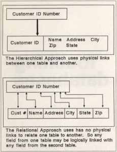
The important word in the last example is logical. Database systems that are not relational link information held in databases with physical pointers, to keep the computer informed as to the whereabouts of each piece of information (see Figure 1). Nonrelational databases are called "hierarchical databases," because of the physical link needed to store information in a database. Because the structure is so rigid, a lot of design and thought must go into a hierarchical database before the actual database is built. Relational databases don't have this limitation.
The origins of a relational database.
The term relational database was originally coined by a man named Dr. E.F. Codd about fifteen years ago. Dr. Codd wrote a standard for a theoretical system called a relational database. At the time, the new standard was developed for large-scale mainframe computers.
Mainframe computers are great for handling large information processing needs; they normally have huge amounts of memory and disk space. Mainframes are still prevalent in large business and industry, but, with the advent of microcomputers, like the Atari ST, small business and even home users can have the utility and power of a mainframe at a reasonable price.
When Dr. Codd wrote the definition of the relational database, twelve rules were defined as a standard to determine if a program was truly relational. Dr. Codd was not a programmer, so when he wrote the definition it was referred to as a model after which programmers should pattern their software. In this article, the term relational model will be used to describe the application of the model. The rules developed by Dr. Codd are very specific in determining ease of use and flexibility of a database program.
The underlying message of the twelve rules is that a database should be able to separate the end user from the actual techniques of handling the contents of the database. When information is stored in a relational database, it's available by means of a common language. The end user enters requests in this common language, and the relational database internally figures out the best possible way of carrying out the user's command.
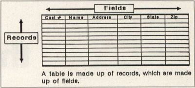
The first rule of a relational database determines how information is logically stored in a table. A table is made up of records. Records, in turn, are made up of a group of fields. This ordering of priorities makes a table look much like a spreadsheet, with fields running left to right as columns, and records running up and down as rows (Figure 2).
The guaranteed access rule states that all information inserted into any table may be retrieved, manipulated or deleted without restrictions. So, if you create a table and store information in it, any information stored may later be accessed, modified or deleted under all circumstances. The hierarchical database links its information with physical pointers, while the guaranteed access rule makes it possible to link information in a logical manner. More on this later.
The SQL language.
The comprehensive data language rule describes the use of a set of common commands that are necessary to manipulate information and control the database. The data language rule shows that the language has to follow some sort of consistent behavior. IBM was one of the first companies to develop a working relational database product. IBM developed the SQL, or Sequel, language. Later, the SQL language was adopted as the industry standard relational database language by the American National Standards Institution (ANSI).
There are two main divisions of the SQL language: query commands and procedural commands. Query commands are those that cause manipulation of the structure of a table or the data stored in a table. Procedural commands control a database program and usually resemble the control commands of BASIC, Pascal or some other high-level language.
Query commands allow you to do two different things. First, you can create, modify or drop a table, thus allowing you to establish the structure of a table or change the structure of an existing table. Second, you can manipulate the information stored in an existing table.
There are four basic query commands to manipulate table information. With them you can:
—Retrieve information already stored in a table.
—Insert new information into a table.
—Update or modify information already stored in a table.
—Delete information stored in a table.
These are the four basic instructions that give you full control over all the information stored in a relational database.
The procedural commands affect the program flow and control of the system. Most of the procedural commands can be found in other high-level languages (such as IF. . .THEN, GOTO and LET.
Data types.
The guaranteed access rule of the relational model states that you can store and manipulate a variety of different types of information. There are many kinds of information. For example:
| Types | Examples |
| Integer numbers | 1, 100, 99 |
| Decimal numbers | 10.01 |
| Character strings | "A person's name" |
| Normal dates | 2/1/86 |
| Short dates | FEB 1, 86 |
| Long dates | February 1, 1986 |
| European dates | 1/2/86 |
The other relational data type is the logical data structure. The logical field contains one of three values: true, false or null. Null indicates that the field doesn't contain a value.
When a table is created, the fields that will comprise every record within the new table are defined. When a field is defined, three facts are stated about the new field: the field's name; the type of field; and how big the field is going to be.
What is the field's name?
A record is made up of fields. When a record is to be added to a table, the predefined fields are assembled into a new record. During this assembly period, each field is referred to by its field name. For example, let's say we're talking about a table that will hold a company's customer address. A typical entry would look something like this:
John Rayston
1313 Harbor Lane
St. Petersberg
Florida
31733
Each line of this address would be entered into a different field. So, the first line is the name field, next would be the address field, and so on. . .
| Field name | Contents of field |
| NAME | John Rayston |
| ADDRESS | 1313 Harbor Lane |
| CITY | St. Petersberg |
| STATE | Florida |
| ZIPCODE | 31733 |
The column to the left contains the field names, while the right column contains the field's contents. If you were to retrieve the zipcode field, it would show 31733.
What is the type of the field?
The relational model can handle many types of fields, like numbers, characters, dates, etc. When new information is put into a table, the field type becomes quite important. There's a big difference between how a date is stored and how a number is stored.
In the example above, two field types were used to store the customer address.
| Field name | Field type | Contents |
| NAME | Character | John Rayston |
| ADDRESS | Character | 1313 Harbor Lane |
| CITY | Character | St. Petersberg |
| STATE | Character | Florida |
| ZIPCODE | Integer | 31733 |
The first four fields are character fields, since both numbers and letters may be used within them. The last field is an integer field, meaning only numbers can be stored. Regent Base support seven field types:
Character...............Any numbers or letters may be used
Integer.......Any whole numbers;i.e., 99, 100, 1, -1
Decimal........Any numbers with a decimal point, i.e., 100.00, 35.99, .25
Date...................A date in this form: 1/1/86
Sdate...A Short Date, shown in this form: JAN 1, 86
Ldate...............A Long Date: January 1, 1986
Edate....................A European Date: 1/1/86 (month/date reversed)
How big is the field going to be?
Every field has a maximum size. If you want to store a person's name within a field, it must fit within the set maximum. For example, if you wanted to store the name JOHN RAYSTON in a name field thirty characters wide, the name field would contain:
John   Rayston
1 2 3 4 5 6 7 8 9 0 1 2 3 4 5 6 7 8 9 0 1 2 3 4 5 6 7 8 9 0
1 2 3
But, if the name field had a maximum of only eight characters, it would look like this:
John   Ray
1 2 3 4 5 6 7 8
Only the first eight characters of the field will be stored. You must define fields that are large enough to handle the data to be stored in them.
Of the seven types of fields, only three must have defined sizes: character, integer and decimal. Character fields can be from 1 to 32,000 characters wide and integer fields can be defined up to 10 digits wide. Decimal fields may also be defined up to 10 digits wide, with up to 10 digits to the right of the decimal point. Date fields are of a predetermined size.
Simple sample example.
Here's a typical example of the field definitions for a table.
| Field name | Type | Size |
| Name | Character | 20 |
| Phone | Character | 20 |
| Age | Integer | 2 |
| 42 Bytes |
This table will hold several people's names, phone numbers and ages. The first is the name field and is a character field, twenty characters wide. Next is the phone field, which is also a character type, twenty characters wide. The age field is an integer field that's two digits wide.
When new information is added to the table, the individual fields are assembled into one record. Let's say we're going to add the following information:
| NAME | John Rayston |
| PHONE | (305) 555-1616 |
| AGE | 35 |
The record might look like this when in the table:
| Name Field | Phone | Age |
| John Rayston | (305) 555-1616 | 35 |
If another person's information is to be added, the new record will be placed at the end of the table.
Applying SQL.
In the last section, we described an imaginary table which would hold three fields of information for every stored record. The query command to create that table would look something like this:
Create Table Phonelist Name Char(20),Phone Char(20),Age Int(2);
This command will create a new table, Phonelist. In it are three fields for every record: name field (up to twenty characters); phone field (also up to twenty characters); and age field (any number, -99 to 99).
Now that a table has been defined, let's see how the SQL query commands work. There are four basic query commands which manipulate information within tables: INSERT, SELECT, UPDATE and DELETE.
Inserting.
The INSERT command adds a new record into an existing table. When a table is created, it initially contains no records. This command adds records, while the other commands retrieve, modify and delete records.
Let's try adding a new record into the Phonelist table. The following command will do this:
INSERT INTO PHONELIST NAME = "John Rayston",
PHONE="(305) 555-1616", AGE=35;
The INSERT command syntax is typical of the English-based format of the SQL language. Once this command has been processed, the Phonelist table will contain one record. Before going on to the SELECT command, let's add another record:
INSERT INTO PHONELIST NAME="Martha Windum,rdquo;,
PHONE="(818) 555-2646", AGE=22;
Thus, the Phonelist table will contain two records for use in the next section.
Selecting.
Now that we have two records in the Phonelist table, we can retrieve the records using the SELECT command. Each record contains three fields: the name field, phone field and age field.
The SELECT command gathers data from certain selected fields in one or more tables. The retrieved information may be displayed on the screen, printed, sent to an output port (i.e., RS232), or used in another SQL command.
The SELECT command has a number of different formats, but all start with one command:
SELECT * FROM PHONELIST;
This is the most basic form of the SELECT command. It will retrieve all (*) fields from the Phonelist table. When this SQL command is processed, the following information will be retrieved:
| Name field | Phone | Age |
| John Rayston | (305) 555-1616 | 35 |
| Martha Windum | (818) 555-2646 | 22 |
Selecting specific field.
When we entered the SELECT command, the * retrieved all of the fields in the Phonelist table. If we wanted to retrieve only the name field, we could substitute the field name for the * character. For example:
SELECT NAME FROM PHONELIST;
This command, when processed, will retrieve only the name field from the phonelist table:
| Name |
| John Rayston |
| Martha Windum |
So far, the SELECT command examples have retrieved all of the records in the table. If we want to be more specific about which records to select, we can add a WHERE clause to a SELECT command.
When processed, the following SELECT command first checks to see if each record meets the WHERE criteria; if a record tests true, it's displayed; if not, it's ignored.
SELECT * FROM PHONELIST
WHERE NAME="John Rayston";
When you process this SQL command, only the John Rayston record will appear.
In addition to a simple check for equivalency (as we just tried in the above example), there are a number of other expressions we can use in the WHERE clause. For example:
˜Contains checks if a phrase or word exists in a field
^ Like checks a field using wildcard characters: * ?
! = Not equals
> Greater than
< Less than
> = Greater than or equal
> = Less than of equal
These expressions can also be used in the other SQL data commands.
You may also use the AND and OR operators within a WHERE clause. For example, suppose we want to retrieve only those records in which a person's age falls between 25 and 40. We could use the following command to perform this function:
SELECT *
FROM PHONELIST WHERE AGE < = 25 AND AGE > = 40;
Processing this command would retrieve the following record:
| Name Field | Phone | Age |
| John Rayston | (305) 555-1616 | 35 |
Arithmetic express in select.
SQL also supports math functions when processing information. Suppose we wish to how old John Rayston will be in 10 years.
| SELECT | name, age+10 |
| FROM | Phonelist |
| WHERE | name5"John Rayston" |
Processing this command would retrieve the following record:
| Name Field | Age |
| John Rayston | 45 |
SQL can also retrieve the youngest person in the table by using the MINIMUM function. This function finds the smallest value for a numeric field.
| SELECT | |
| FROM | phonelist |
| WHERE | age=MIN(AGE) |
Processing this command would retrieve the following record:
| Name Field | Phone | Age |
| Martha Windum | (818) 555-2646 | 22 |
Updating.
Once a record has been inserted into a table, it can be modified using the UPDATE command. This command allows you to specify the fields and records to modify.
We previously added two records to the Phonelist table. Using UPDATE, we can change either of these two records. For example, let's say we want to change both phone numbers to 555-2244. The following command will do just that:
UPDATE PHONELIST SET PHONE= "555-2244";
When you process this SQL command, the contents of the phone field in all records of the Phonelist table will be changed to the new phone number in the UPDATE command.
To see if the Phonelist table really was changed, enter the following SELECT command:
SELECT * FROM PHONELIST;
This will retrieve the two records in the Phonelist table as shown below. Notice that both phone fields are now equal to 555-2244.
| Name Field | Phone | Age |
| John Rayston | 555-2244 | 35 |
| Martha Windum | 555-2244 | 22 |
When we processed the last UPDATE, every record in the Phonelist table was modified. Like the SELECT command, UPDATE may also use the WHERE clause.
Using the WHERE gives us a lot of flexibility. If we wanted to change the Phone field of Martha's record, we could use an UPDATE WHERE command like this:
UPDATE PHONELIST SET PHONE="555-9512"
WHERE NAME="Martha Windum";
When this is processed, the contents of the phone field in the Martha Windum record will be changed to the new phone number.
Deleting.
Now that we know how to INSERT, SELECT and UPDATE, the last function to accommodate the guaranteed access rule is the DELETE command, to remove a record from a table.
There are two forms of the DELETE command: DELETE and DELETE WHERE. The former allows us to delete everything from a specified table, and the latter allows us to delete specific records from a specified table.
If you were to process the following command, every record in the Phonelist table would be deleted:
DEELETE PHONELIST;
Using DELETE WHERE, we can delete the Martha Windum record from the Phonelist table:
DELETE PHONELIST WHERE NAME="Martha Windum";
The real power.
So far, we've described the most primitive functions of a relational database using the SQL language. The real power of a relational database is in its flexibility. The SELECT command allows us to treat the information stored in a table as individual objects. The logical pairing of these objects of information is where the relational database shows its greatest power.
For example, let's say we have two tables which contain information about certain customers of a company. The first table, Custinfo, has two fields: Customer, which holds the customer number; and Name, which holds the customer's name.
| Table: CUSTINFO | |
| CUSTOMER | NAME |
| 1010 | John Sinkley |
| 1020 | Fred Barnes |
| 1030 | Mary Hartner |
The second table, Accounts, has two fields: Customer, which holds the customer number; and Amount, which holds the amount owed to the company.
| Table: Accounts | |
| CUSTOMER | AMOUNT |
| 1020 | $ 30.00 |
| 1030 | $132.00 |
| 1010 | $ 5.49 |
The SELECT command is able to produce a report showing each customer's number and the amount owed. For example:
This command finds every record in both tables where the Customer fields in both tables hold the same name. The results of this command would be:
| 1010 | John Sinkley | $ 5.49 |
| 1020 | Fred Barnes | $ 30.00 |
| 1030 | Mary Hartner | $132.00 |
This form of SELECT performs an algebraic function called "intersection." The intersection of the two tables is the common Customer field. The relational database logically produces the intersection of the two tables, based on the conditions of the WHERE clause.
Conclusion.
This article is by no means a complete description of all the power and functionality built into the relational database model; but it's a good jumping-off point.
The relational database model was previously restricted to large-scale mainframe computer systems. The relational approach to databases, though, is gathering momentum in the microcomputer world. Companies such as Ashton Tate, which produces dBase II and dBase III Plus, have announced relational products. Other companies already have a relational database on the IBM PC, like Microrim's RBASE System V.