THE PET® GAZETTE
Contour Plotting
Neal E. Reid
Parkside High School,
Dundas, Ontario
In the July/August issue of COMPUTE (p. 73) John Winn showed how to use the 2022 printer to produce graphs of functions of one variable, f(x). Two features of the printer made it possible to increase the resolution from that of a printed character to that of a single printer matrix dot. First of all, the user can define special characters to print any one of the matrix dots alone in the character space. Secondly, because of the variable line spacing on the printer, the character and thus the matrix dot can be printed anywhere on the paper.
The object of this article is to show how to produce graphs of functions of two variables, f(x,y). I am using a 2023 friction feed printer which does not have the variable line spacing capability. As a result, gaps sometimes appear in the plotted lines, but these are readily filled in by the eye and do not seem to be a serious defect.
One cannot approach the problem of graphing a function of two variables in the same way that one does a function of a single variable. In f(x,y), x and y are both independent variables. A particular pair (x,y) represents a point in a plane and the value of the function represents heights above or below the plane. I like to picture f(x,y) as a physiographic map. X and y correspond to distances in the east-west and north-south directions, respectively. The function corresponds to the elevation at a particular point (x,y) on the map. Points at which the value of the function is zero are at sea level. Positive values of f(x,y) are above, negative values, below sea level. To represent such a function on a two dimensional sheet of graph paper, one plots lines of equal elevation-contour lines. A line connecting the points where f(x,y) = 0, for instance, would be the shore line on a physiographic map. It is customary on such a map to show a constant change in elevation from one contour to the next. Then in regions where the contour lines come very close together, the slope of the land must be very steep - moving a short distance horizontally changes the elevation a great deal. Alternatively, if the contour lines are very widely spaced, then the terrain is relatively flat.
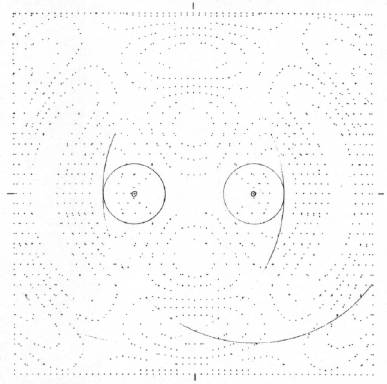
INTERFERENCE OF TWO CIRCULAR WAVES
RANGE OF X: -6 TO 6 X-INCREMENT: .2
RANGE OF Y: -6 TO 6 Y-INCREMENT: .337333333
CONTOURS: 1.5  .9 .3 -.3 -.9 -1.5
PLOTTING TIME: 40.4 MIN
In setting out to draw contours of a function of two variables, the first things to consider are the scale and the position of the graph. The position is fixed by choosing the center of the graph to be at some particular point (X0Y0) in the xy plane. Then by adjusting the scale, one can display a large area or a small neighborhood of that point. Giving the width XR of the graph from the center to the edge will fix the scale. This restricts x and y both to a limited range of values. Thus it is not necessary to print out the graph standing on its side in order to let x have an unlimited range as is usually done with functions of a single variable.
The physical size of the final graph depends on the number of characters per line and the number of lines printed, and this in turn determines the values of the increments in the x and y directions. The printer character matrix is 6 dots wide and 7 dots high with a 3-dot spacing between the lines. By choosing the dimensions of the graph to be 60 characters wide and 36 lines long, we end up with a 360×360 dot square, 6 inches on a side, which fits nicely on an 8½×11 sheet of notebook paper. The boundary of this region is made using a special character MK$ consisting of the single dot in the upper left hand corner of the print matrix. It is printed around all four sides of the square. Moving across the page, the x increment, the change in x from one dot to the next, is XR/30 (center to edge width/30 characters). If the graph boundary were a perfect square, then the y increment would be XR/18. On my printer, however, the vertical dimension comes out about 1/16 inch longer than the horizontal. For truly precision work, one should correct for this; thus, the peculiar factor in line 1035 arrived at purely by trial. The scale, increments, etc., are all taken care of in the SET UP subroutine starting at line 900. The increments and ranges of x and y are printed out at the end of the plot. With this information, these dots on the boundary provide an accurate scale for the final graph. In addition, there are tick marks on the edges to locate the exact center of the graph.
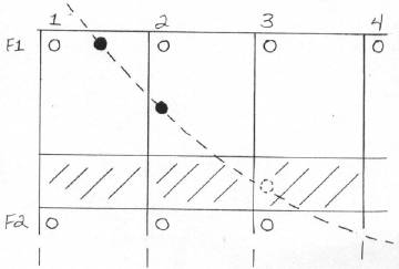
The procedure to create a contour plot for a given function is now straightforward. First, values of the function are calculated at points spaced uniformly over the entire page using the increments of x and y previously worked out. Then we examine every pair of points to see if the contour passes between them. The points at which the function is calculated are those corresponding to the dot in the upper left hand corner of each character. Actually this is done only one line at a time in the subroutine beginning on line 400. After finishing two lines, we have the situation depicted in the diagram. The open circles are the points at which the value of the function is now known.
To find out if the contour we are interested in cuts through the space occupied by the first character, we test to see if the value of the contour lies between the values Fl(1) and F2(1) on the horizontal line. This test is made in line 600. If the test is passed, then the particular dot at which the contour cuts the top edge of the matrix is found by linear interpolation. This test is repeated in line 610 for the vertical line between F1(l) and F2(1). Each character space is examined in the same manner, and whenever a contour crossing is found, a dot is printed on the left and/or top edge of the matrix. Dots on the left edge which fall into the space between two lines cannot be printed. Other dots in the matrix are never printed. When the first line of characters is completed, the functional values in F2 are shifted into F1 and the next line of values is put into F2. This way the program never requires more than two lines of values in memory at any one time.
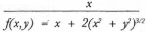
I have used the function f(x, y) = x2 + y2 as a sort of test pattern to check out the program. The contours of this function are circles centered at the origin. The accuracy in the positions of the plotted points can be checked with a compass. (The user should check this for himself.) If the width XR is set equal to 3 and the contour values are taken to be 0.25, 1.00, 2.25, 4.00, 6.25, and 9.00, then the radii of the circles differ by ½ inch from ½ to 3 inches.
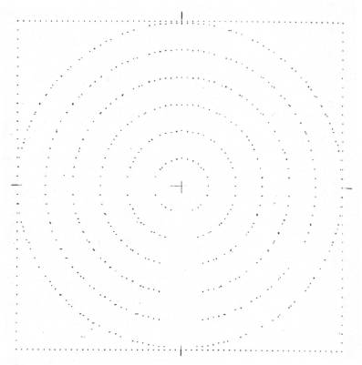
TEST PATTERN - CONCENTRIC CIRCLES
RANGE OF X: -3 TO 3 X-INCREMENT: .1
RANGE OF Y: -3 TO 3 Y-INCREMENT: .168666667
CONTOURS:	   .25 1 2.25 4 6.25 9
PLOTTING TIME: 23.9 MIN
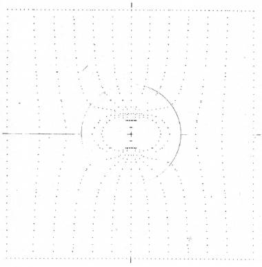
FLUID FLOW AROUND A SPHERE
RANGE OF X: -2.5 TO 2.5 X-INCREMENT: .0833333333
RANGE OF Y: -2.5 TO 2.5 Y-INCREMENT: .140555556
CONTOURS:	    2 1.6 1.2 .8 .4 0 -.4 -.8 -1.2 -1.6 -2
PLOTTING TIME: 38.6 MIN
The user should set his own function equal to F2(J) in line 440.
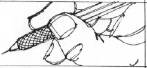
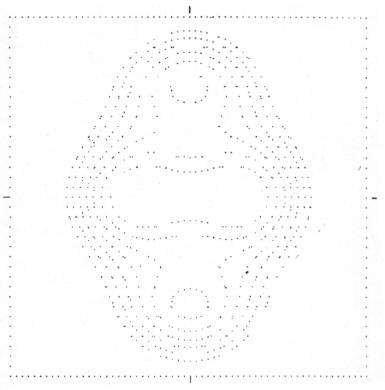
The second diagram is an example of a typical contour plot. It shows the equipotential lines in the magnetic field of a bar magnet. The north pole of the magnet, which has been drawn on the plot, is at x = -1. The south pole is at +1. The potential at an arbitrary point in the plane is given by the function.
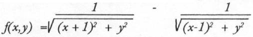
The lines of force start at the north pole, end at the south pole, and are everywhere perpendicular to the contours. The program does not label the contour lines, but it is not difficult to figure out which is which. For one thing you can plot one contour at a time until you see where they lie. In this plot the contours increase toward the left from zero on the y axis to .1 which is the innermost one. They decrease to the right. The plotting time increases with the complexity of the function and with the number of contours. Each plotted point requires an excursion of the print head across the page.
One potential source of trouble is the possibility of a division by zero. In this plot, for instance, this could happen at the positions of the poles. In fact, around the north pole there is a peak which becomes infinitely high at the pole, and at the south pole there is an infinitely deep hole. (Notice the cliff between the poles where the contours coincide!) In practice it is a simple matter to select the center of the graph and the scale so as to avoid having to evaluate the function at these troublesome points. The point (.00001, .00001) is indistinguishable from the point (0, 0) to the eye but it makes a difference to the computer.
This plotting routine can be used for any relationship that can be expressed as a function of two variables. Some examples which the reader might find interesting to try out are given below. I am sure there are many others. On the other hand, it is of great interest just to experiment with functions of all sorts and see what turns up.
- Interference of circular waves. Two pebbles are dropped into a pond at the points x = +2 and -2. Draw circles of radii 1 and 5 around these points on the finished graph. These show where the peak of each circular wave lies. Maximum values of the function occur where two of these circles intersect. The wave troughs are half way in between at radii of 3 and 7.

Center: (0,0) Width: 6
Contours: 1.5, .9, .3, -.3, -.9, -1.5
- Fluid from around a sphere. (Draw a circle of radius 1 on the finished plot.) The contours are lines of the velocity potential. The flow of the fluid is from right to left. The stream lines of the flow are everywhere perpendicular to the contour lines. Near the sphere they hug the surface.
Center: (0, 0) Width: 2.5
Contours: 2.0, 1.6, 1.2, .8, .4, 0, -.4, -.8, -1.2, -1.6, -2.0
- The distribution of matter in the nucleus of Neon-20. This is what you could expect to see if you could slice open the nucleus like an apple.

Center: (0, 0) Width: 2
Contours: 1.4, 1.3, 1.2, 1.1, 1.0, 0.9, 0.8
DISTRIBUTION OF MATTER IN NEON-20
RANGE OF X : -2 TO 2  X-INCREMENT :  .0666666667
RANGE OF Y : -2 TO 2  Y-INCREMENT :  .112444444
CONTOURS :   1.4 1.3 1.2 1.1  1  .9 .8
PLOTTING TIME  33.2 MIN
50 REM * * * * * * * * * * * * * *
51 REM *                         *
52 REM *     CONTOUR PLOTTER     *
53 REM *                         *
54 REM * * * * * * * * * * * * * *
60 :
61 REM NEAL E. REID
62 REM PARKSIDE HIGH SCHOOL
63 REM DUNDAS, ONTARIO
100 :
101 REM MAINLINE
110 GOSUB 900 : REM SET UP
120 PRINT#1, TAB(31)"%" : GOSUB 800
130 LN = 0 : PRINT "↓ LINE NUMBER : ↓↓"
140 GOSUB 400 : REM COMPUTE F2
150 LN = LN + 1 : PRINT "↑" LN
160 FOR I = 0 TO 60 : F1 (I) = F2(I) : NEXT
170 GOSUB 400 : GOSUB 500
180 IF LN < 36 GOTO 150
190 GOSUB 800 : PRINT#1, TAB(31) "%"
200 :
210 PRINT#1 : PRINT#1
215 PRINT#1, TL$ : PRINT#1
220 PRINT#1, "RANGE OF X: " ; X0 - XR;
230 PRINT#1, " TO " ; X0 + XR;
240 PRINT#1, "			   X-INCREMENT : " ; XI
250 PRINT#1
260 PRINT#1, "RANGE OF Y : " ; Y0 - XR;
270 PRINT#1, " TO " ; Y0 + XR;
280 PRINT#1, "			  Y-INCREMENT : " ; YI
290 PRINT#1
300 PRINT#1, "CONTOURS :	" ;
310 FOR K = 1 TO NC
320 PRINT#1, CT(K) ;		: NEXT
330 PRINT#1 : PRINT#1
340 T% = (TI - TM)/360
350 PRINT#1, "PLOTTING TIME : " ;
360 PRINT#1, T%/10 ; " MIN"
370 CLOSE 1 : CLOSE 5
380 PRINT "PLOT COMPLETED"
399 END
400 :
401 REM CALCULATION OF FUNCTIONS
402 REM ON 60X36 GRID
403 REM ONE LINE AT A TIME
404 REM COORDINATES ARE (X, Y)
410 Y = Y - YI
420 FOR J = 0 TO 60
430 X = XS + J * XI
440 F2(J) = X^2 + Y^2
450 NEXT J
499 RETURN
500 :
501 REM PLOT CONTOURS
510 REM BOUNDARY AND X MARKER -
520 PRINT#5, MK$
530 IF LN<> 19 THEN PRINT#1, SP$SC$TAB(59)SC$CR$;
540 IF LN = 19 THEN PRINT#1, "#"SC$TAB(59) SC$"#" CR$;
550 REM LOCATE CONTOURS -
560 FOR J = 0 TO 59
570 A = F1(J) : B = F1(J + 1) : C = F2(J)
580 FOR K = 1 TO NC : NV = 0 : NH = 0
590 CN = CT(K)
600 IF A < = CN AND CN < B OR A > = CN AND CN > B THEN NV = INT(6 * (CN - A)/(B - A)) + 1
610 IF A < = CN AND CN < C OR A > = CN AND CN > C THEN NH = INT(10 * (CN - A)/(C - A)) + 1
620 IF (NH = O OR NH > 7) AND NV = 0 GOTO730
630 REM CREATE SPECIAL CHARACTER -
640 A1 = 2 ^ (7 - NH) : IF NV = 1 THEN A1 = A1 + 64
650 A2 = -64 * (NV = 2)
660 A3 = -64 * (NV = 3)
670 A4 = -64 * (NV = 4)
680 A5 = -64 * (NV = 5)
690 A6 = -64 * (NV = 6)
700 A$ = CHR$(A1) + CHR$(A2) + CHR$(A3)
705 A$ = A$ + CHR$(A4) + CHR$(A5) + CHR$(A6)
710 PRINT#5,	  A$
720 PRINT#1,	  TAB(J + 1)SC$CR$;
730 NEXT K
740 NEXT J
799 PRINT#1 : RETURN
800 :
801 REM PRINT BOUNDARY
810 PRINT#5, MK$
820 PRINT#1, SP$;
830 FOR I = 1 TO 61
840 PRINT#1, SC$; : NEXT
850 PRINT#1, CR$;
899 RETURN
900 :
901 REM SET UP
910 DIM F1(60), F2(60), CT(12)
920 DATA 64, 0, 0, 0, 0, 0
930 FOR I = 1 TO 6 : READ A
940 MK$ = MK$ + CHR$(A) : NEXT
945 INPUT "ĥTITLE" ; TL$
950 PRINT "↓X, Y COORDINATES OF"
960 INPUT "CENTER OF PLOT" ; X0, Y0
970 INPUT "↓CENTER TO EDGE WIDTH" ; XR
980 INPUT "↓NUMBER OF CONTOURS" ; NC
990 PRINT "↓CONTOUR VALUES:↓"
1000 FOR K = 1 TO NC
1010 INPUT CT(K) : NEXT
1020 XI = XR/30	  :REM X-INCREMENT
1030 XS = X0-XR	  :REM X INITIAL VALUE
1035 YR = XR * 1.012
1040 YI = YR/18	  :REM Y-INCREMENT
1050 YS = Y0 + YR :REM Y INITIAL VALUE
1060 Y = YS + YI
1070 SP$ = CHR$(29)  : REM SPACE
1080 SC$ = CHR$(254) : REM SPEC. CHAR.
1090 CR$ = CHR$(141) : REM CAR. RETURN
1100 OPEN 1, 4 : OPEN 5, 4, 5
1110 PRINT "↓INSERT PAPER"
1120 PRINT "↓PRESS rRETURN&rcirc;";
1130 PRINT " TO CONTINUE"
1140 GET P$ : IF P$ = " " GOTO 1140
1150 IF ASC(P$) <> 13 GOTO 1140
1160 TM = TI      : REM SET TIMER
1170 PRINT "↓STARTING"
1199 RETURN