ON DISK!
ST SCIPLOT
by David P. HeddIe
Do you need to produce precision graphs on your ST for scientific or technical work? ST SciPlot is your solution! START's ultra sophisticated graphing program is for use in universities, labs or wherever super-quality precision graphs are needed. Runs in high resolution monochrome only.
Plot your data precisely! SCIPLOT.ARC is on your START disk.
Business graphing programs are becoming more common on the ST, but if you have wanted to put the ST's power to work for you in the lab, you were out of luck. ST SciPlot is START's solution to your power graphing problems. Written in Personal Pascal, ST SciPlot is a full-featured GEM application that produces the kind of graphs found in technical literature. It requires the high resolution of the ST's monochrome monitor--sorry, color monitor owners!
Features
Some of the features that distinguish ST SciPlot from the ordinary graphing programs are:
- Each axis can be set to a linear or logarithmic scale
- The X and Y-axes are interchangeable and vertical and horizontal error bars can be included.
- Up to four plots, each with up to seven curves, can be displayed at the same time using six line types and six marker types.
- You can create your own font set or use (and edit) the default set which includes the full Greek alphabet and a mathematical symbol library.
- The fully editable and draggable text display includes optional legends, titles, annotations and axis and date/time labels, all with available superscripts and subscripts.
- Connecting lines can be linear or you can use the built-in cubic spline generator for smooth curves.
- Simple ASCII data sets may be loaded, edited or deleted or you may enter data directly.
Getting Started
ST SciPlot is in the archived file SCIPLOT.ARC on your START disk. To un-ARC ST SciPlot, copy SCI PLOT.ARC and ARCX.PRG to a blank, formatted disk and follow the Disk Instructions located elsewhere in this issue. Once you have un-ARCed SCIPLOT.ARC, double-click on SCIPLOT.PRG. The file SCIPLOT.FNT must be in the same directory as SCIPLOT.PRG.
A few definitions are necessary here for you to make the best use of ST SciPlot. A plot is a single set of up to seven curves. A plot environment is the full definition of all of the settings for a particular plot, including location, scaling, labels, line styles, etc. An active plot is the plot you have selected for modification; only one plot may be active at a time.
The Menus
When you boot ST SciPlot, you will see a menu bar with the headings as shown in Figure 1. Also shown in Figure 1 are all of the drop-down menus with their choices. Let's run through these menus.
The Action Menu
- Read Raw File--loads a set of raw data in ASCII format, replacing the current data set for the active plot. ST SciPlot uses a default filename extender of .DAT, although this is for convenience only. See below for how to set up a data file.
- Read Saved File--loads an ST SciPlot file with an .SPT filename extender, replacing the current data and plot environment. These files include the definitions of all of the plots at the time the file was saved, whether or not you had actually defined four plots.
- Input By Hand--allows you to enter data manually into the grid shown in Figure 2. The number of columns is the number of data sets and the number of rows is the number of data points per set; any empty boxes within a data set will be set to 0 (zero) by ST SciPlot.
- Save Data--Saves the current data and plot environments in ST SciPlot format. While no filename extender is required, .SPT is recommended.
- Save Image--Saves a snapshot of the current ST SciPlot screen in DEGAS high-resolution format. Be sure to add the .P13 extender.
- Plot--Plots the current data on the active plot using the current plot environment.
- Plot Boxes Only--Draws only the outline boxes and the labels without actually plotting any curves. This is useful for checking the locations of your plots without taking the time to actually draw the curves.
- Print--Prints the current screen. You can set your printer and paper type from the selector box called by this menu item.
- Defaults--Restores ST SciPlot environment defaults. A confirmation dialog box prevents you from resetting your environment accidentally.
- Quit--Quits ST SciPlot, again, with confirmation.
The Active Menu
There are four menu choices: Plot 1 Active, Plot 2 Active, Plot 3 Active and Plot 4 Active; you may choose one of these plots to be active (modifiable).
The Style Menu
The Style Menu uses toggles (on/off switches) to select style attributes. If a checkmark appears by the attribute, that style is selected.
- Markers--Places a marker at each data point.
- Lines--Places a connecting line between adjacent data points.
- Legend--Displays the legend.
- Legend Box--Draws a box around the legend.
- Title Box--Draws a box around the title.
- Error Bar Ends--If you use error bars, this will place small, perpendicular lines at the ends of the error bars.
- H-Zero Line--If the Y-value range includes 0, this places a horizontal, dashed line through Y=0.
- V-Zero Line--If the X-value range includes 0, this places a vertical, dashed line through X=0.
- Full Plot Box--Draws a rectangle around a plot; otherwise, draws only the axes.
- Date & Time--Displays the date and time at the time it is selected.
- Order Data--Orders (organizes) the X-axis data before plotting. Should be selected, unless you want to plot "parameter" plots.
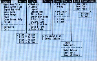 |
| Figure 1. The ST SciPlot menu bar and the drop-down menus with their selections. |
The Fitting Menu
- Straight Line--Uses a straight line to connect adjacent curve points.
- Cubic Spline--Uses a natural cubic spline to connect adjacent points on a curve, but takes more time to plot than Straight Line.
The Axes Menu
- X-Linear--Makes the X-Axis scale linear.
- X-Log--Makes the X-Axis scale logarithmic, unless the minimum X-Axis value is negative. If it is, ST SciPlot will use X-Linear.
- Y-Linear--Like X-Linear, but on the vertical axis.
- Y-Log--Like X-Log, but for the vertical axis.
- X Label--Allows you to generate and edit the label for the X-Axis.
- Y Label--Like X Label, but for the Y-Axis.
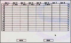 |
| Figure 2. This is the manual input data grid. The number of columns is the number of data sets and the number of rows is the number of data points per set. |
The Review Menu
- Title--For editing the Title.
- Data Sets--Brings up the Data Set box shown in Figure 3 for editing of data set names, scale factors, axis limits, etc. See below for further discussion.
- Data Values--Displays the data sets in tabular form.
- Edit Data--Displays the data sets in grid format. Click on a box to select that value for editing, then enter a new value. Click on the row number to add a new row to be inserted with values of zero for each point. Click on the asterisk (* ) at the right end of a row to delete that row.
- Special Chars--Displays the complete character set and the keystroke equivalents needed to generate the special characters. See Figure 4.
The Font Menu
- Load Font--Loads a new font file. Note, however. that ST SciPlot font files are not standard GEM font files and you will get an error message if you try to load one. Font files for ST SciPlot must be generated within ST SciPlot.
- Save Font--Saves the current font file to disk. While the .FNT filename extender is not mandatory, it is recommended. On boot-up ST SciPlot will read in the file SCIPLOT.FNT.
- Edit Font--Allows you to edit the current font. Selecting Edit Font will bring up the font grids shown in Figure 5. Pressing a key selects that character for editing. The top left grid shows the character, the top right shows the backslash (\ ) character and the bottom two grids show the subscript and superscript versions. You edit a character by toggling individual pixels on or off with the left mouse button; you can see the actual character as you are editing it in the small box below the editing grid.
The Annotations Menu
- Strings--Allows you to enter up to ten lines of annotations per plot and specify their locations on the screen. Selecting Strings will bring up the Strings screen shown in Figure 6. See below for further information.
- Arrows--Brings up the Arrows screen (shown in Figure 7) and allows you to add up to ten arrows with open or closed arrowheads and specify the beginning and ending positions of the arrows on the screen.
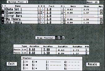 |
| Figure 3. The Data Set box allows you to edit the names of your data sets, the scale factors, the axis limits, the marker and line styles and data set axis assignments. |
Data Files
As mentioned above, ST SciPlot allows you to load in an ASCII data file. Each such "raw" data file can contain the curve data for a single plot. If you load in a raw data file using the Read Raw File option on the Action menu, it will replace the data in the active plot with the new data. You may generate your own raw data file using any text editor or word processor that has an ASCII or "Print to Disk" option.
Each raw data file consists of a series of rows of numbers with each value delimited (separated) by a space and each row terminated by a carriage return. Each column is a set of values and all the columns together are a data set. You may have no more than eight columns per data set and each column must have the same number of items. You may interchange entire rows or columns freely without generating errors. However, by default, ST SciPlot does assign the first column as the X-Axis data set and the others as Y-Axis sets, but this may be changed in the Review Data Sets screen. (See below.)
Don't worry if you have more values in one column than another; simply pad the short column out with any arbitrary value so that the columns all have the same number of values. After loading in that set of values, you can specify the number of values to be used (Np) for that set. See below for more on editing data sets.
You may use integer, decimal or logarithmic (base 10) numbers in your data sets. For example, see Figure 8. This data file contains four data sets (columns) with five entries for each of the first two sets and three "real" entries for the last two sets and two padded values of zero.
Editing Data Sets And Data Display
There are two aspects of editing data sets: you can edit the data itself directly through the Edit Data selection on the Review Menu or you can edit the display of that data through the Data Sets selection on the same menu. The first alternative has been covered above.
The Data Sets Review screen is shown in Figure 3. All entries shown in the larger system font can be edited; all entries shown in the smaller custom font can not. The boxes at the top show which plot is active and how many data points it contains. The first column identifies the data sets; any Y-Axis data sets in inverse video will be plotted. Click on the set number to toggle it on or off.
The second column tells the type of data set, X-Axis (X), Y-Axis (Y) or Error Bars (E); click on each of these boxes to cycle through the choices. The third column contains the first 20 characters of the 60-character data set name that will appear in a legend. To change a name, click on it and edit it in the dialog box.
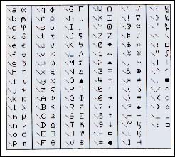 |
| Figure 4. In addition to the upper- and lowercase English alphabet and Arabic numerals ST SciPlot has a complete Greek alphabet, plus an extensive mathematical symbol library. |
The fourth, fifth and sixth columns apply to Y-Axis data sets only. In order, they are X-Axis (X), Vertical Error (V) and Horizontal Error (H). Clicking on each of these boxes allows you to specify which of the other sets will be used for the X-Axis values, the vertical error values and the horizontal error values for that curve. If you choose a hyphen (-) in the X column, that curve will not be plotted.
The seventh column is the Factor (Fact) column. By clicking in any box in this column, you can change the scaling factor for that data set. The scaling factor is always applied to the original data, not to the data as previously scaled.
The next two columns, Marker Style (M) and Line Style (L), allow you to choose the style for that data set from the choices shown in the chart at the bottom of the screen. Just click on each to cycle through them until you have the one you want.
The next two columns can't be edited. They show the maximum and minimum values for each data set.
The last column shows the number of data points used to plot each curve. The maximum is Ndat, but you can select any number less than that by clicking on the appropriate box and typing in the new value.
In the middle of the screen is the Draw Plot(s) bar. Curve numbers shown in inverse video are plotted; they can be toggled on and off by clicking on them.
Below the Draw Plot(s) bar is the Axis Limit grid. You can change the Maximum and Minimum values for each axis (and the resultant scale of the plot) by clicking on them and entering new values. The labels are self-explanatory, but you must keep the maxima equal to or greater than the largest value in the data sets and the minima equal to or less than the minimum values in the data sets. If you attempt to set a maximum or minimum axis value that is within the data range, ST SciPlot will set that value to equal the limit value (highest or lowest).
The column to the farthest right is labelled Ntk. The values in this column (Number of Tick Marks) determine where the divisions are marked along the axes. ST SciPlot has an internal heuristic algorithm that determines values for these parameters. It attempts to minimize "waste" and to choose Ntk so that the divisions occur at "nice" places. The maximum value for Ntk is 6; you can choose any lesser value by repeatedly clicking on the appropriate box to cycle through the choices.
There are two boxes to the left and right of the Styles chart; to the left is the Exit box (self-explanatory) and to the right is the Recalc box. If you click on the Recalc box, ST SciPlot will recalculate the axis limits using its internal algorithm.
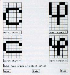 |
| Figure 5. You can edit each character in ST SciPlot's custom font set. The top left grid shows the character, the top right shows the custom character and the bottom two grids show the subscript and superscript versions. |
Editing Text Strings
ST SciPlot allows a variety of text strings to be displayed on a plot and all of them can be edited. The X- and Y-Axis labels are edited through the X Label and Y Label selections on the Axes Menu. The Plot Title can be edited through the Title selection on the Review Menu. The curve names can be edited through the Data Sets selection, also on the Review Menu.
As noted above, ST SciPlot uses a custom character set, which can be reviewed through the Special Chars selection on the Review Menu. In addition to the upper- and lower-case English alphabet and Arabic numerals, ST SciPlot has a complete Greek alphabet, plus an extensive mathematical symbol library. (See Figure 4.) All of these special characters are accessed through a two-character sequence beginning with a backslash (\ ); this is the key just to the right of the Return key.
ST SciPlot can also display text in normal, superscripted and subscripted modes. To change to superscripted mode, type a caret (^ ) before the string by holding down the [Shift] key while pressing the number 6 key in the top row of the keyboard. To change to subscripted mode, type an underscore (_) in front of the string by holding down the [Shift] key while pressing the hyphen key. To return to normal text mode, type a vertical bar ( | ) by holding down the [Shift] key while pressing the backslash key.
Annotations And Arrows
ST SciPlot also allows you to add up to ten lines of annotations of 60 characters or less each and specify their locations on the screen. When you select Strings on the annotations Menu, the Strings screen appears, as shown in Figure 6 and you may enter your annotations for the active plot.
Under the title bar on the Strings screen are ten lines for entering the text of your annotations. Each line may be up to 60 characters long and you may use the custom character set, superscripts and subscripts. Click on the line you wish to edit and then enter the text. As with all text or numerical entry boxes in ST SciPlot, you may use the [Escape] key to clear the entry or the [Delete] or [Backspace] keys in their usual manner.
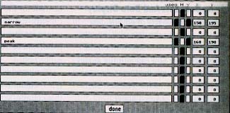 |
| Figure 6. From this Strings screen, you can specify up to ten lines of annotations and place them anywhere on the graph, either vertically or horizontally. |
To the right of the text lines are four columns of boxes. The first is labelled "used"; click here for each line of text you wish to display on the graph. A black box indicates that the text will be shown on the screen. Next to the used column are the "v" (for vertical) and "h" (for horizontal) columns; click on one or the other of these to specify the direction you want the text to run.
The next two columns are for the horizontal (x) and vertical (y) starting position of the text. This is specified in pixels, counting down and to the right from the upper left-hand corner of the screen. The usable area for a single character is from 0 on the left to about 630 on the right and 20 at the top to about 390 at the bottom. Click on each box to enter your setting. The default is set to 0; after you have brought up the entry box, be sure to clear it by pressing the [Escape] key.
After you have entered your annotation strings and set their location and direction, click on the "done" box to return to ST SciPlot's main screen. The Annotations may not be visible. If they aren't, just re-plot the graph. If they still aren't visible, return to the Strings screen and check that the used boxes are highlighted for the annotations you want to display and that the x and y locations are within the ranges specified above.
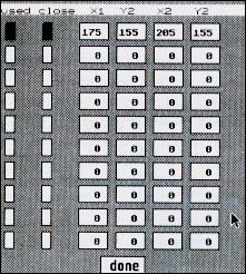 |
| Figure 7. The Arrows screen allows you to specify up to ten arrows with either closed or open arrowheads anywhere on the screen. You specify their location by entering the pixel locations where you want the arrows to begin and end. |
Clicking on the Arrows selection on the Annotations Menu brings up the Arrow screen shown in Figure 7. From this screen, you can specify the position and arrowhead style of up to ten arrows for use with your annotations. There are six columns on the Arrows screen; the first is labelled "used" and operates just like that on the Strings screen. Just click on each box to turn that arrow on.
The next column (close) allows you to specify the arrowhead style. If the box is black, the arrowhead will have a triangular arrowhead. If the close box is white, the arrowhead will be drawn in the standard open drafting style.
The next four columns allow you to set the horizontal and vertical position of the "tail" of the arrow (x1 and y1) and the horizontal and vertical position of the "head" of the arrow (x2 and y2). These are specified in pixels, just like the string location. Again, be sure to press the [Escape] key to clear the default 0 setting before entering your numbers.
It may take a bit of practice to determine the exact locations for your annotations and arrows. Just remember that X=0, Y=0 specifies the upper left-hand corner of the screen and that the values increase as you go from left to right and from top to bottom. Also, remember that the annotations and arrows are specified in absolute screen locations and can not be dragged with the mouse. To change their locations, you must reenter the Strings or Arrows screens and change the values there; also, re-sizing or moving your plot will not relocate the annotations or arrows.
|
|||||
| Figure 8. ST SciPlot can read this mixed data set with no trouble. It contains four data sets (columns) with five entries in each of the first two sets and three "real" and two padded values of zero in the last two sets. |
|||||
Dragging And Sizing
Labels, titles and the time string can all be dragged around the plot to a new location by clicking anywhere within the text and dragging it in the usual GEM manner (just like dragging a Desktop icon). To drag a legend or an entire plot, first make sure that the plot is active and then drag it or the legend with the mouse, just as with the text strings. If you click outside a plot or any label, the active plot will flash.
There is an invisible GEM sizing button diagonally outside the lower right corner of each plot rectangle. If you wish to resize a plot, click within this sizing button and hold the left mouse button down. A sizing rectangle will appear and you can then size the plot just as with a GEM Desktop directory window.
Error Messages
As with any feature-intensive program, ST SciPlot will generally prevent you from attempting the impossible. Here are some common error messages: Can't find Font File: SCIPLOI.FNT--The font file must be in the same directory as SCIPLOT.PRG on booting. Data Too Close to Spline Setting to Linear Fit--If the data points are too close together, using a cubic spline could produce an error. Try interchanging the X-Axis and Y-Axis data sets. Illegal Scaling Factor. No Scaling Performed--Scaling factors must be greater than 1.0E-20 and less then 1.0E+20. Input Error. No Data Read.--Something is wrong with the data file format. No Consistent Data.--You have made a mistake in the Data Sets Review screen that prevents a meaningful plot. For example, you may have set all data sets to be Y-Axis values.
Conclusion
As you can see, ST SciPlot is immensely powerful. Space just doesn't allow a full discussion of all of its features; yet ST SciPlot is so logically designed that each of your questions can be answered by an examination of the context in which it arises. Also, there is nothing like experimentation--you can't hurt your computer or the program by trying anything and everything ST SciPlot allows. Once you've worked through a plot or two and read through this article thoroughly, the interface will be second-nature to you. And then you can put your ST to work in your lab!
David Heddle is a physicist at the University of Illinois and a consultant for Booz, Allen & Hamilton, Inc.