The Digital Magnet
BY DAVID SMALL
This spectacularly colorful graphics program simulates magnetic field line generation. If you are more interested in detail than color, you can also run it on a monochrome system; it works in any resolution. Related files may be found within the MAGNETS folder on your START disk.
I guess magnets have always fascinated me. As a kid, I loved to play with iron filings and magnets, electromagnets, and whatnot.
One day in freshman physics we were discussing formulas governing magnets. I woke from my usual haze just enough to note the formulas and think, "This would make a neat program. At our local computer center, there were two unused Tektronix 4013 graphics terminals hooked up to a Cyber mainframe, so I spent some time on them and wrote the original Magplot, a magnetic field lines plotter.
The program wasn't a waste of time. After all, it helped me pass my freshman physics class. It also earned a reputation for pulling computer time out of the mainframe; when I ran the program, I could hear the chatter of teletypes in the next room slow down, sometimes stop, a result of all the floating point arithmetic going on.
Well, enough history. Let's look at the program.
THEORY
The formula for attraction hetween two charged particles is:
(CHARGE1 * CHARGE2) / (DISTANCE SQUARED)
Or, the attraction repulsion between two objects is dependent on their distance squared. You'll find this same relationship in other popular formulas, such as for gravity.
With multiple particles, you must calculate the force exerted at any point by summing up the charges exerted on each point by each particle. The easiest way to do this is to calculate each force as a vector, then add up the vectors. You end up with a vector which, at a given point, represents the sum total of the attraction/repulsion being exerted on it at that point.
This is similar to figuring out the direction a satellite will go by summing up the relevant gravitional pulls from all the bodies (the sun, planets).
If you then draw a small line in the direction the vector points, recalculate the attraction/repulsion, and so on, you will obtain a picture of the field lines around magnets. If you've ever done the experiment with iron filings and a magnet, the plots done by this program will look remarkably familiar.
Two like forces will repel each other; you'll see the field lines reflect this, as the " +" and "+" points repel one another. Opposite forces attract, again, you'll see the field lines traveling from + " to "-".
There's also a physics theorem that field lines plotted this way will never cross one another. This is the case in the program.
PROGRAM
The program was originally written in Cyber BASIC, and over the years has ended up on an amazing variety of graphics-oriented computers. The ST and C language are the latest target, and one of the faster implementations; the 68000 and C seem to be pretty adept at floating point arithmetic, which this program spends a vast amount of time doing. You will see a certain amount of BASIC within the code in this incarnation of the program, including the entirely global variables. Please feel free to optimize it. Quite honestly, the original program took me so long to get working properly under BASIC, I have a mental block about playing with it too much.
The program has three main sections. The first involves initialization and setup of controlling variables. Since the ST's processor is not infinitely fast, there are some practical limits to make the plot occur reasonably quickly. I've set these up as easily tweaked variables in a procedure called initglobals; feel free to play' around with them. Here's the rundown:
A) linelength: This is how far a line is drawn in a given vector's direction. Too long, and the smooth curves of the field lines will become jagged; too short, and the CPU will spend too much time calculating between points.
B) clipit: This variable, if found to be True, 'clips" field lines to the size of the screen; in other words, if you're drawing a field line and it goes offscreen, the line is terminated. The problem here is that offscreen lines are pure CPU calculation and the wait on them can get pretty tedious; on the other hand, most plots look far more complete if you include the off-screen line. If you select no clipping, then the line is terminated only if it goes wildly out-of-hounds and has little chance of returning on to the screen area.
C) degreeinc: The starting point for each line is on a circle around positively charged points. The line then travels to a negative point, by whatever route, or gets terminated off-screen. degreeinc determines the degree increment between starting lines. The lesser this variable, the more lines are plotted off each positive point; on the other hand, it takes longer to generate a given plot. If you make this variable very low, you'll have quite a dense and good looking plot, but it will take awhile to generate.
D) k2: This is a miscellaneous force constant that determines how much strength a magnetic field has. If you've ever wanted to play god and turn off magnetism, here's your chance. The value is more or less kludged to make good plots.
E) radius: This value determines the "black hole" radius around a negative point and also determines the starting radius of each positive point.
The second section of the program lets you input the charge points using the mouse. This is done primarily within inputpoints(). Admittedly, it is a bit kludgy, but it does not require resource files or calls to the AES. This shortens and simplifies the program, particularly if you don't have the Resource Construction Set.
When the mouse button is pressed during point input, the point's X and Y locations are recorded, and a "menu" for positive/negative is displayed. Click on either POS or NEG to select that point's charge. I store the X,Y, and charge of the point in three arrays, xcoord, ycoord, and (creative name) charge.
The "menu" is then erased.
When you press [Shift] or [Alternate], you exit the while loop that inputs the points, and proceed to the program's third main section which deals with plotting the picture.
PLOTIT()
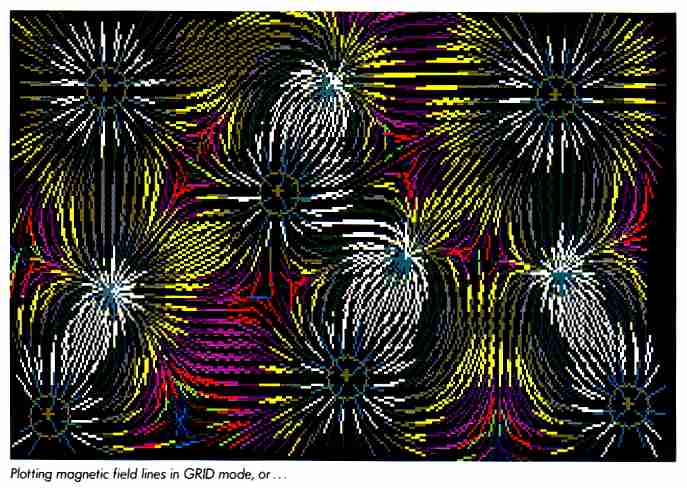
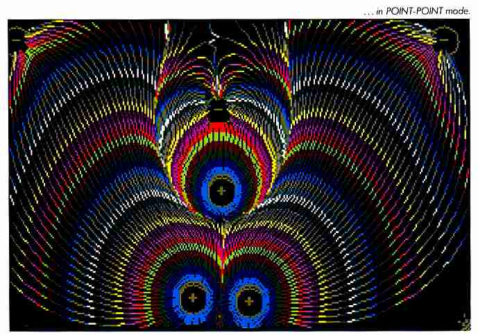
There are two ways of creating the picture. One gives a fairly accurate picture of the field lines by plotting continuous lines, the other a good-looking plot by plotting one line on a grid overlaying the picture area. I include both; you select which one you'd like with the gridstyle option. If you want the grid approach, exit the point-input process with [Alternate]; if you'd like the point-point approach, use [Shift].
In grid mode, we start at all X's and Y's forming a grid on the surface, calculate the line direction at that particular point, draw the line, and move to the next point. The line's color is drawn based on the amount of force present at that particular point (the vector summation), which makes for a spectacular display in low or medium-resolution.
In point-point mode, we run several nested loops. In order, they are: 1) Cycle through all positive points; 2) Start a line at N points around each positive point; 3) Sum charges at each point; draw the line.
The charge summer is set up as a separate call to make grid plotting easier. The CPU spends most of its time here, as the variables are double floating point, required because of the fractions involved. You'll find the distance between points being calculated as sqrt ( (xl-x2) squared + (yl-y2) squared ). You'll also find the basic force equation here.
The charge summer inputs the point as x1, y1 (old BASIC variable names) and outputs the next point on the line, scaled to linelength, in the same variables.
VDI's v_pline (polyline draw) then draws the line and proceeeds to the next point.
CONSIDERATIONS
There are some interesting practical considerations that I ran into when designing this program.
How should the lines start in order to create an even plot? This was solved by using polar coordinates around each positive point. (You can't begin a line at a negative point because it travels towards the nearest negative point-itself.)
How do you terminate the line? This was not trivial. It is easy if the line goes offscreen, but, when the line nears a negative point, there is a "black hole effect"; the distance is so short that the negative point becomes the only relevant force. The line is drawn one linelength past the negative point, which causes it to overshoot the negative point; it then turns around, overshoots, and so forth, creating a ping-pong effect.
The solution here is to terminate a line whenever it becomes radius close to any negative point. This stops the ping-pong effect. Regrettably, it involves calculating the distance to every negative point on each line draw, which involves extra CPU time; perhaps a simpler solution would be a subtraction against each negative point's coordinates.
What if the line goes offscreen? There is special code to handle this case, if you decide to let the line wander offscreen and return. The variable newline "initializes" the line for subsequent v_plines so you don't get a strange skipping effect.
There are some miscellaneous routines to make the plot work on any style monitor. The high-res monitor, of course, gives the cleanest picture, but there are only two colors, black and white. The two color modes allow some interesting possibilities for color and animation. I cycle through the color register numbers (either 0-3 or 0-15) while drawing the force lines, and the result is a pleasing multi-color force line; if the color registers are then rotated 'underneath" the plot, so to speak, the force lines become animated, travelling from positive to negative points. You'll see the rotation code in the line drawing routine.
As the code notes, the GEM color number seldom corresponds to the extended BIOS call hardware color number. This caused me some trouble, and I had to include a fair amount of code just to deal with this problem.
You might find the "POS/NEG" code to be useful in writing resolution
independent codes. I calculate all the X and Y constants on the basis of
character width and screen size returned from the VDI "open workstation"
call.
HOW TO RUN MAGPLOT
1. Double click on the program's file icon, MAG21.PRG. Once the program is loaded, the top screen will read: Exit: (SHIFT=pt-pt; ALT=grid). At this point, pressing [Shift], [Alternate], or [Control] will exit you to the Desktop.2. Click the mouse anywhere on the screen where you would like a point, then click on either POS or NEG to select that point's charge. Continue inputting points like this until you have as many as you like. A quick demo is two points-one positive and one negative-a distance from each other on the screen.
3. Having chosen your points, press [Alternate] to plot in GRID mode, [Shift] to plot in point-point mode. Try both to see the difference. During the actual plotting-or when finished, you may restart by pressing [Shift], or exit the program by pressing [Control].
MAG21 works in all resolutions but is flashiest in lowres. On color monitors, the program will color-cycle at the end of point-point mode.