Statistics For Nonstatisticians
A. Burke Luitich
Basic statistical methods can help you make logical decisions in everyday situations.
For the most part, elementary statistical methods measure a group of similar things to see how these measurements vary when compared to some standard. Another use for statistics is to see how creating a group of objects can cause variations in these objects.
This program, "Statistics," takes your raw data and returns figures which you can use to make everyday decisions, for example, about the best way to build a wall or how much cash you'll need when you go shopping.
As a first example, let's look at two ways to cut a 2 x 4, by using a power table saw and a handsaw. We set the table saw guide to one foot and cut a five pieces. We cut five more pieces using a handsaw, then measure the actual lengths of all ten pieces to see how accurately we made the cuts.
If nothing unusual is allowed to affect the cutting, we can expect the length of the pieces to vary depending on the process used. Statisticians call this an unbiased random sample.
Assume the measurements are as follows:
| Table saw lengths | Handsaw lengths |
| (feet) | (feet) |
| 1.05 | 1.22 |
| .95 | .91 |
| 1.03 | .80 |
| 1.07 | 1.28 |
| .96 | .88 |
The Same Mean
A look at the values alone suggests that cutting with the handsaw is a far less consistent method than using the table saw. However, if you add up the lengths for each method and divide by 5 (the total cuts for each) you will find that both methods give the same mean (average) length of 1.018 feet.
Just finding an average length doesn't tell us much. What we need to know is how widespread the values are likely to be, and which method gave us the most lengths that were nearer our standard of one foot. In statistical terms, we need to calculate the range and the standard deviation.
We find the range by subtracting the shortest length from the longest, for each cutting method. For the handsaw the range is. 48 feet (1.28—.80), and for the table saw the range is .11 feet (1.07—.96). Immediately, we can see that the table saw cut more consistently, because the range, or variation, is smaller.
We can use the standard deviation and the mean length to predict how often a given length is likely to occur. You don't have to worry about how to calculate a standard deviation; the program does this for you. If you type in the above lengths for the handsaw, the program will return a standard deviation of .217 feet. The standard deviation for the table saw is .047 feet.
Degree Of Accuracy
If we made a large number of cuts, then measured and graphed the lengths, the graph would form a bell curve, or normal distribution. By combining the standard deviation and the mean length, we get a range of lengths that includes 68.3 percent of all lengths (again, you don't have to know the theory; just use the number). To illustrate, first take the mean length, 1.018 feet, and subtract from it the standard deviation for the handsaw, .217 feet, to get .801 feet. Then add the standard deviation to the mean length to get 1.235 feet. This means that 68.3 percent of our lengths fall in the range between .801 and 1.235 feet.
By adding and subtracting the standard deviation (.047 feet) with the mean length of the table saw cuts (1.018 feet), we find that 68.3 percent (roughly two-thirds) of these lengths fall in the range from .971 to 1.065 feet.
If you want a wider sample, you must increase the number of standard deviations. To include 95.4 percent of all lengths, use two standard deviations. For the handsaw, we now have .434 feet, two standard deviations. Combining it with the mean length, we get a range of .584 to 1.452 feet. Our table saw range becomes .924 to 1.102 feet (1.018 plus and minus .094).
Food For Thought
You can use the same methods to calculate a food budget. In this case, your data consists of the amounts you spent on groceries over a 13-week period (one-fourth of a year):
| Week | Amount | Week | Amount |
| 1 | $42 | 8 | 47 |
| 2 | 50 | 9 | 65 |
| 3 | 75 | 10 | 49 |
| 4 | 37 | 11 | 43 |
| 5 | 51 | 12 | 52 |
| 6 | 45 | 13 | 54 |
| 7 | 56 |
If you type this data into the Statistics program, you will find that your mean amount spent was about $51; that your spending varied from $37 to $75, for a range of $38; that you spent more than $50 (your median amount) as often as you spent less than that; and your standard deviation is about $10.
Applying The Statistics
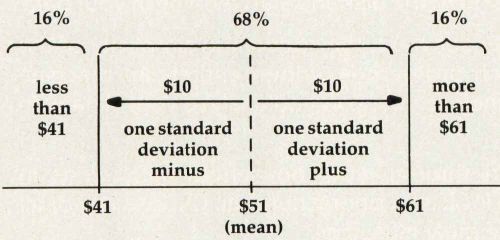
Combining one standard deviation and the mean (or average) amount spent, we find that two-thirds of the weeks you spend between $41 and $61 at the grocery store. One-sixth of the time you spend less than $41; one-sixth of your bills are more than $61. So, if you budget $61 for groceries, you'll have enough 84 percent of the time.
If you want to be sure you'll have enough in case prices rise, you might want to use two standard deviations. By adding two standard deviations ($20) to the mean amount ($51), you will find that, to be about 98 percent sure, you should budget $71 each week.
There are other factors to be considered, of course, such as vacations, birthday parties, or visiting relatives, that can affect your food budget. The Statistics program does not take these kinds of things into account. But it does give you a tool which takes some of the guesswork out of everyday decision-making.
The Statistics program requests input of the size of the sample, or number of items to be entered (line 410), then requests the values of the sample measurements (lines 500–550). All the statistics referred to in this article are then calculated, that is, mean, standard deviation, median, and range.
Lines 325–350 and 4900–5610 give the user a thumbnail sketch of the information to be calculated and a description of each of the statistics. While the sample size is limited to 100 for the VIC version (other versions allow up to 300), this should be more than adequate in most cases.
Error Correction
An error correction routine is included in lines 555–580 and 5900–6190. This provides for the change of any entry before the calculation. While the program is running, a delay of up to two minutes will be experienced while the program performs several sorts on the data. This is normal for BASIC and may be longer for sample sizes in the 80 to 100 range or greater.
Program 1 requires at least 3K of expansion memory in the VIC computer. If the instructions, error correction routine, and headings are eliminated, the program will run on an unexpanded VIC. Specifically, the following lines should be deleted if the program is to run without memory expansion: 95–180, 325–350, 555–580, 4900–5610, and 5900–6190.
Further reductions can be made by reducing the sample size, redimensioning the array in line 90 to the new sample size (SA), and changing the value of 100 in line 420 to the new maximum sample size.
Statistics for a sample of 100 readings requires about 30–45 minutes to calculate by hand. This program requires about 8–10 minutes, including input.