VIC Scaling Bar Graphs
James P. McCallister
Bar graphs often have more visual impact than figures or statistics. This utility program gives you multicolor bar graph capability and demonstrates its practical uses. There is a discussion of modification of control variables to suit a variety of applications.
As you learn to solve problems in BASIC on your VIC, you realize that calculations are fairly easy to program no matter how complex the math. However, you sometimes want to display your answers in a way that highlights their meaning. One very effective method is to construct a bar graph.
This article describes a utility bar graph subroutine you can add to your own programs. It's very easy to use, and it's suitable for many applications. Once you have it saved on tape or disk, you can quickly turn a modest calculation into an analysis of options or a graphic history of trends.
One Practical Application
Here's an example that demonstrates a practical use of the bar graph subroutine. Suppose you want to borrow money to buy a car. Checking a reference book on business math, you find that the monthly payment calculation for an installment loan is:
payment = amount of loan * r/(l-(l + n)-r)
where n is the number of months and r is the monthly interest rate, expressed as a decimal fraction. Also,
total finance cost = (n * payment) - amount of loan
So, as a first step, you come up with this BASIC program to do the fundamental calculation:
100 INPUT "{2 DOWN} AMNT, APR"; AM, AR
110 MR = AR/1200
120 INPUT "MONTHS"; N
130 MP = AM * MR/(l-(l + MR) ↑ - N)
140 FC = N * MP - AM
150 DEFFNR (X) = - INT ( -X * 100)/100
160 PRINT "PAYMNT = $"; FNR (MP), "FIN COST = $"; FNR (FC)
170 GOTO 100
In this program, AM is the amount of the loan, AR is the annual percentage rate, and N is the term, in months. MR is the monthly rate expressed as a decimal fraction. The results are MP, the monthly payment, and FC, the total finance cost; both are based on the formulas you started with. The function FNR (X) defined in line 150 rounds to the next highest penny, and the results are printed in line 160.
Naturally, increasing the number of months (or term) of the loan makes the payment lower, but increases the finance cost. With this program you could experiment with various amounts, APRs and terms, and arrive at a decision about which loan suits you best.
Instead, let's modify the program to plot the effect of various term lengths of the loan, using the bar graph subroutine. We'll still use the INPUT statement for amount and APR; but we'll use the FOR/NEXT statements to automatically vary N and take care of storing the answers. Now the program looks like this:
100 INPUT "{CLR} AMNT, APR"; AM, AR
110 MR = AR/1200
120 FOR I = 0 TO 8 : N = 6 * (I + 2) : REM N = 12 TO 60 BY 6'S
130 Y (0, I) = AM * MR/(l-(l + MR) ↑ - N)
140 Y (1, I) = N * Y (0, I) - AM
150 NEXT I : QB = 8
160 QL$ = "{12 SPACES} l 2 3 4 5 {15 SPACES} YEARS"
170 QT$ = "{2 SPACES} MONTHLY PAYMENT" : Z = 0 : GOSUB 9900
180 QT$ = "{2 SPACES} TOTAL FINANCE COST" : Z = 1 : GOSUB 9900
190 GOTO 100
Add lines 9900 to 9999 (see Program 2).
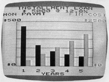
The resulting graphs are in Figures 1 and 2 for a loan of $5000 at 12.8 percent.
We'll deal with the new variables in detail later. But you can already see that plotting the graphs requires these steps:
- The BASIC instructions for the subroutine are added to the program, beginning in line 9900. (Later, we'll discuss the most efficient ways to do this.)
- The numbers to be plotted are put into two lists, one for each graph. At line 130, the list for the monthly payment graph is put in Y (0, I), and at line 140 the list for the finance cost graph is put in Y (1, I). The first subscript for each Y variable identifies the list. The second subscript is a label for each number in the list.
- After the lists are completed, GOSUB9900 is "called" once for each graph (line 240).
- Before calling GOSUB9900 the first time, QB is given a value of 8 so the subroutine would know how long the lists were and how many bars to plot. Also, the legend to appear at the bottom of the screen is put in QL$.
- Before calling GOSUB9900 each time, title information is put in QT$. This is different for each graph.
- Before calling GOSUB9900 each time, Z is given a value corresponding to the list to be plotted.
The graphs in Figures 1 and 2 can be displayed using just the lines listed so far. The subroutine does all the layout work. The vertical scale and labeling are automatic. The example could have included billions of dollars or 10-9 seconds of time – the scale would still be worked out and labeled correctly.
Program Features
Now we're ready to explore the features of the subroutine in greater depth. The primary features are:
•one to 21 vertical bars per display (number specified by user).
•automatic ranging and scaling for each display, with no restrictions on the signs or magnitudes of the values to be plotted. The scale is labeled.
•operates from a two-dimensional array, so that several lists can be stored before plotting the first one.
•positive bars go up; negative bars go down.
•built-in "hold" of display, released by touching any key; cursor prompt in lower-right corner.
•universal memory configuration. Adds 2300 bytes to the calling program.
•scale lines in contrasting color (green).
The subroutine also has a number of optional features which are transparent to the user. (Transparent features are built-in program features that you can ignore without consequence – they take care of themselves.) The features are controlled by giving values to certain control variables. In BASIC, all numeric variables are initially set to zero, and the subroutine is designed so that a zero signifies the standard condition for each option. That's why the standard choices are transparent. The standard choice for an option is often called the "default" option, because if you don't specify an option, you'll get the standard choice by default. The transparent features are:
•The top four lines of the display can be printed with title or explanatory information. (Null strings are standard.) Also, the two bottom lines can be printed with legend information.
•Choice of bar color (black is standard); or contrasting colors for "up" and "down" bars; or alternating bar colors; or contrasting colored bars grouped in pairs.
•Close-spaced (standard) or double-spaced bars.
•Graph positioned against right edge of screen (standard), or moved left a chosen number of spaces.
•Automatic ranging and scaling, with all bars starting at zero (standard); or expanded, offset scale; or preassigned scale. Also, pre-scaling of multiple lists before plotting.
•Vertical scale labeled (standard), or unlabeled. Labels are printed to the left of the scale, if there's room. Otherwise, they will move automatically to just above or below the scale.
How To Use The Subroutine
To create a bar graph plot, insert GOSUB9900 into your program after assigning the value or values to be plotted into the Y array. There are two fundamental restrictions in your main program. First, you cannot use line numbers from 9900 to 9999. Second, you shouldn't use variable names starting with Q, unless you're willing to share them with the subroutine.
The result of the GOSUB9900 (if no control variables are set) will be a single bar, representing the value stored in Y(0,0). Going beyond this simple graph requires using control variables – but only those you want to change from zero. Most likely you'll find that several of the controls are quickly mastered. You can then add more to your repertoire as you gain experience. All control variables must be given any new values before GOSUB9900.
Optional Feature Controls
These are the rules for the control variables:
- List identification. The variable Z becomes the first subscript of the Y values, thereby controlling which list is to be plotted. If there is only one list, then Z is always zero and never needs to be changed from its initial zero value.
- Number of bars. The number of bars plotted is controlled by the variable QB. QB = 0 plots one bar; QB = 1 plots two bars, etc. The maximum value of QB is 20, which will plot 21 bars scaled to the values stored in Y(Z, 0), Y(Z, l), Y(Z, 2) – up to Y(Z, 20). If either Z or QB is greater than ten, it is mandatory to use a DIM statement at the beginning of the program to DIMension the Y array. Even if they are both less than ten, it's still good programming to DIMension to save memory.
- Title and legend. Up to 88 characters of title can be printed on the top four lines by creating a string variable QT$. Likewise, up to 44 characters of legend can be printed on the bottom two lines with QL$. [Note: The 44th character of QL$ can be used only with a trick. For example, if the last word is MONTH, end QL$ with the sequence "...MONH {LEFT} {INST}T". Otherwise, the top of the display will roll up and off. This sequence is only needed for exactly 44 characters.]
- Bar color options. Bar colors are controlled with the standard VIC POKE codes for colors (which are one number lower than that color key on the keyboard). For example, the code for black is zero, and black is the standard color for the bars. The color control variables are Q0 and Ql. By assigning nonzero values to one or both, you can do the following:
- Bar spacing. The standard option provides bars which are closely spaced. However, if QB is assigned a negative value, the bars will be plotted with a space between them. The maximum negative value allowed is ten (QB = -10), which will plot 11 bars separated by 10 spaces. In addition, if the alternating bar colors option is chosen at the same time that QB is negative, the bars will be plotted in closely spaced pairs separated by open spaces. Under these conditions, the maximum negative value allowed is 13 (QB = -13), which will plot seven pairs (14 bars) separated by six spaces.
- Graph centering. The graph is normally positioned against the right edge of the screen (standard). You can move it to the left n spaces by setting QC = n.
- Scale factor options. The options for the automatic ranging and scaling feature are controlled by the variable QS. The standard choice, QS = 0, will always produce a useful graph of the data, and in many cases the result can't be improved upon. However, sometimes a bar graph can be done in a different way that makes it more informative. After all, effective chartmaking will always consider the reader, the data being compared, the most significant facts, and so on. The optional choices for QS allow you to have a scale offset from zero, or a prespecified scale. You can also prescale lists of values before doing any plots, which is desirable for merged graphs or for finding a common scale for several graphs in sequence.
•All bars one color: assign the same color to Q0 and Ql. Example: Q0 = 6 : Ql = 6 will result in all blue bars.
•Up bars one color, down bars another: assign the color for the up bars to Q0, and the color for the down bars to Ql. Example: Q0 = 0: Ql = 4 will result in black bars pointing up and purple bars pointing down.
•Bars alternating colors: if either Q0, Ql, or both are given a minus sign, then ABS(QO) is the color of the even bars and ABS(Ql) is the color of the odd bars. Example: Q0 = 6: Ql = -7 will result in bars alternating between blue and yellow.
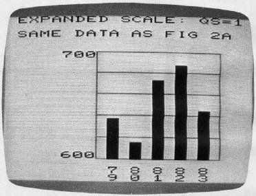
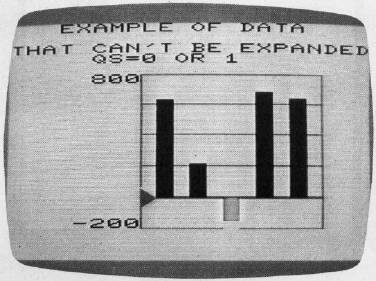
Figures 3 and 4 illustrate the scale offset from zero. The graph in Figure 3 results from QS = 0. Depending on the circumstances, this may be the best graph for this data. One problem, however, is that the variations are small compared to the length of the bars. If the variations are the most important characteristic of the data, then Figure 4 is a better display. This is achieved by making QS = 1. The scale is expanded as much as possible – times ten, in this case. It must also be offset so the bottoms of the bars don't reach zero.
If you were the chairman of a charity sale and this was a graph of yearly results, you'd probably use Figure 4 when talking to your committee because it's easy to see the changes. But you might use Figure 3 in the final report because it doesn't exaggerate the bad news for '83. In Figure 4, the bar for '83 is only 50 percent as high as '82, but Figure 3 shows the true proportion – 93 percent. An offset scale isn't always possible, as, for example, when the list includes both positive and negative numbers. In such cases, QS = 1 will not have any special effect on the graph. Figure 5 is a graph of such data.
The QS = 2 option allows you to second-guess the Automatic Ranging and Scaling Rules by giving starting values to QX and QN. These two variables store the maximum and minimum values found in scanning the list of numbers to be plotted. This option, in effect, allows you to preassign a particular scale or a particular offset. Study the rules under "Automatic Ranging And Scaling," and then experiment to master this option.
The prescaling options, QS = 3, 4, and 5, are the same as QS = 0, 1, and 2, except nothing is put on the screen. But the maximum value (QX), minimum value (QN), scale factor (QZ), upper-scale label (QU), and lower-scale label (QD) are all computed and made available to the main program. Our final program uses this capability to combine Figures 1 and 2 into one graph. It's possible to make some very effective displays with these options, without a lot of programming.
- Scale labels. You can suppress the printing of the scale labels within the subroutine by making QS negative, or if QS = 0, by giving it a value of-.l.
Putting It All Together
Now we're ready to demonstrate some of these optional features using the car loan example. Program 1 merges the two previous bar graphs (Figures 1 and 2) into one display using two bar colors (see Figure 6).
Line 90 dimensions the Y array to conserve memory. If we don't do this, the BASIC interpreter will DIMension it Y(10,10) by default and tie up 455 extra bytes of memory.
We discussed lines 100–150 in the car loan example. Lines 160–190 prescale the Z = 0 and Z = 1 lists and then create a merged list suitable for graphing on a common scale. The merged list, in Z = 2, contains both monthly payment and finance cost data, but at twelve-month intervals, instead of six. After prescaling each old list, the values are divided by their respective scale factors for combining into the new list. As a result, the numbers in the new list are all in the range of 0 to 5, instead of their true values. Therefore, we suppress the printing of the automatic scale labels and overprint with the labels (QU) obtained during the prescaling calls. As you can see, line 160 prescales the Z = 0 list, and line 170 prescales Z = 1. Line 180 puts five Z = 0 values into the Z = 2 list, with subscripts (2,0), (2,2), (2,4), (2,6), and (2,8). Line 190 puts five Z = 1 values into subscripts (2, 1), (2, 3), (2, 5), (2, 7), and (2, 9).
Line 200 establishes the optional features for the bar graph by assigning values to control variables Z, Ql, QB, QS, and QC. You should be able to match up the values in the program with the features in the graph.
Lines 210–230 create the string variables for the title and legend. Notice that part of the title uses the input variables for the amount and APR of the loan.
The scale labels we need for this graph are special, so the subroutine labels were turned off. In line 9988, you can GOSUB to your own subroutine and overprint the graph with anything you wish. In our program, we GOSUB 800–830.
Adding The Subroutine To Your Program
There are several ways to use this program with your own programs, but the easiest is to plan ahead. If you want bar graph displays, load this program into memory before you start to type in your main program, and you've got it. However, if you want to combine the bar graph subroutine with a program that's already on tape or disk, without retyping the program, here's a technique to do this which should work every time. It's a slight embellishment of Mark Niggemann's method (COMPUTE!, March 1983, p. 210).
Let's assume that you have a copy of the bar graph subroutine (Program 2) saved on tape or disk with a filename "BARSUB", and that you have a main program we'll call PROGA also saved. You want to improve PROGA by adding bar graph capability. First of all, the program cannot have any line numbers as high as BARSUB's line numbers. That is, they must be below 9900. In the case of Program 1 in this article, you must be sure to delete line 9988 before going further. LOAD PROGA and observe the line number restriction. Then clear the screen and type:
?PEEK(43),PEEK(44)
RETURN and write down the two answers, which make up the start-of-BASIC memory pointer. On an unexpanded VIC, they'll be 1 and 16 (location 1 on page 16). The trick is to change the Start pointer to be two less than the current value of the End pointer in 45 and 46. A reliable way to do this is to type in the following in direct mode (no line number) and hit RETURN:
A = PEEK(45) + 256 * PEEK(46) - 2 : B = INT(A/256) : POKE43, A � 256 * B : POKE44, B
Then proceed:
LOAD"BARSUB"
PRESS PLAY ON TAPE
OK
SEARCHING FOR BARSUB
FOUND BARSUB
LOADING
READY.
Finally, POKE the numbers you wrote down back into memory. For the unexpanded VIC, for example:
POKE43, 1 : POKE44, 16
At this point you have combined the two programs and are ready to proceed with debugging.
A Look At The Program
The bar graph subroutine adds 2300 bytes to the main program. That's not including the Y array and the part of the main program that gets ready to call the subroutine. Even so, a worthwhile program will still fit in a 5K unexpanded VIC. Our final example, which generated Figure 6, left 205 bytes free after RUNning. To keep the subroutine memory size to 2300 bytes, be sure to omit all REMarks and spaces (except inside quotes) when typing the program.
Figure 1: Car Loan Analysis - Monthly Payment
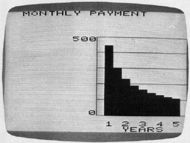
Figure 2: Car Loan Analysis - Total Finance Cost
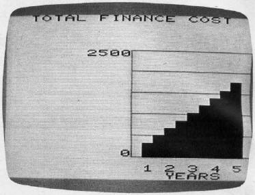
Figure 3: Standard Scale
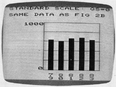
Figure 4: Expanded Scale With Offset
Automatic Ranging And Scaling Rules
The bar graph subroutine follows a set of automatic ranging and selling rules in the process of making the graph. The entire scale consists of six lines outlining five intervals. The value represented by one interval is called the scale factor. For example, in Figure 4 there are six lines representing 600, 620, 640, 680, and 700. Each interval between lines represents 20, which is the scale factor.
These are the rules the subroutine follows to decide on the scale factor and the values for the scale lines:
- The maximum value, QX, is the most positive, or failing that, the least negative value in the list of bars. Likewise, the minimum value, QN, is the most negative, or. Failing that, the least positive.
- The scale factor will be 1, 2, or 5 times 10n where n is a positive or negative integer, or 0. (If n is 0,10n is 1.) Typical scale factors would be 5, .02, 1000, 1E-6.
- The values of the scale lines must be multiples of the scale factor, or zero.
- The scale factor will be the smallest number possible, so that the full scale will include the maximum and minimum values, QX and QN. For the standard scale option, QS = 0or 3, the full scale must include zero. Therefore, QX and QN are given starling values of zero before scanning the list of Y values.
- For Ihe QS = 1 or 4 option. QX and QN will be given a starting value equal to Y(Z, 0) before the maximum /minimum scan. This will result in an expanded scale, with three exceptions:
- If QS = 2 or 5, the values of QX and QN at the time of GOSUB9900 are carried into the subroutine, and the rules are followed on that basis. This allows you to choose your own scale factor or offset. However, if the data in the list won't fit your scale, the scale will automatically be changed to fit the data.
•If all Y values are identical, an expanded scale is possible, but the automatic rules can't decide on one.
•If the Y list contains both positive and negative values, the scale cannot be expanded.
•If the maximum and minimum values are already spread out over the normal scale, the scale cannot be expanded.
In these cases, the subroutine will work as if QS = 0 or 3.