How Random Are Sequences Of Random Numbers?
Brian J. Flynn
Vienna, VA
Chance is a word void of sense; nothing can exist without a cause.—Voltaire
Editor's Note: RND is one of the more intriguing aspects of computers: how do you generate accidents in a world dedicated to logic? Though Mr. Flynn analyzes the TRS-80 RND here, his approach and methods are applicable to any RND analysis.—RM
You turn on a Model I TRS-80 and key in "PRINT RND (0)." The response is "768709." You key in the same command. The response this time is "781397." You do this again, and again, and again. Using a FOR NEXT loop, suppose you generate a "random" sequence of 1,000 numbers. Or perhaps you generate 10,000. Or maybe even 100,000. Have you ever wondered how such "random" sequences of numbers are?
Before performing a statistical experiment a short while ago, I wanted to make sure the TRS-80's random number generator was a good one. So I examined its degree of randomness using a few popular statistical tests and a few common sense indicators.
But before discussing these, first note that the phrase "a random number" is used popularly to denote a member of a "random sequence" of figures. Strictly speaking, however, the adjective "random" should modify only "sequence," unless we happen to be concerned with the digits which comprise a number. This is because 0.768709 is not any more or any less random than 0.5 or 0.372 or any other positive fraction. Each occurs with zero probability in the selection of one number from the infinitely dense continuum of fractions from 0 to 1.
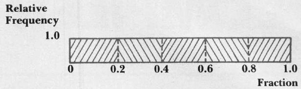
Executions of RND (0) on the TRS-80 generate rational numbers between 0 and 1, inclusive. "Rational," in this case, does not mean sensibility, but rather means that the fraction is expressible as a ratio of two integers. For instance, 0.625 is equivalent to ⅝. And the "rational" number 0.768709, from above, equals 768709 divided by one million. Fractions generated by RND (0) are supposed to be distributed in roughly uniform fashion as in Figure 1. Almost as many fractions should fall between 0 and 0.1 as between 0.1 and 0.2, and so on.
How close to uniformity are distributions of TRS-80 fractions? From machine-off to machine-on position, 100,000 executions of RND (0) generate the spread shown in Table 1. Non-TRS-80 owners may want to use the BASIC program listed here to see how well the random number generators on their machines compare.
The distribution in Table 1 is highly, but not perfectly, uniform. Less than perfect uniformity, however, is desirable. For if exactly 10,000 figures fell into each category, then the mechanism that generated this spread would seem awfully mechanical, too good to be true. While a good random number generator may father a perfectly uniform distribution, the probability of this is very low.
Just how close to uniformity should the distribution of fractions be? The chi (pronounced "ki") square goodness-of-fit statistic provides an answer:
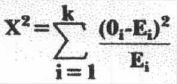
is the Greek capital letter sigma, for sum; k is the number of categories, also called cells or intervals; 0i is the number of fractions observed in the ith interval; and Ei is the number expected. In our case, K = 10 and Ei = 100,000/10 = 10,000.
Let's reveal the mystery of the formula. First, 0i-Ei is the deviation of the expected from the actual number of observations for category "i.". Next, this deviation is squared because (0i-Ei) = 0. Finally, the squared deviation is divided by Ei to give equal importance to each category in cases where the Ei's are different from one another. To clarify this last point, let E1 = 500 and E2 = 1,000 for the two-interval case. If 01 and 02 are 10% higher than E1 and E2, respectively, then(01-E1)2 = (550 - 500)2 = 2,500 and (02 - E2)2 = (1,100 - 1,000)2 = 10,000. The second squared deviation is four times the first. Now, weighting each squared deviation relative to expected number, (01-E1)2/E1 = 2,500/500 = 5 and (02 - E2)2/E2 = 10,000/1,000 = 10. The second term is now only twice as large as the first, just as E2 is twice as large as E1.
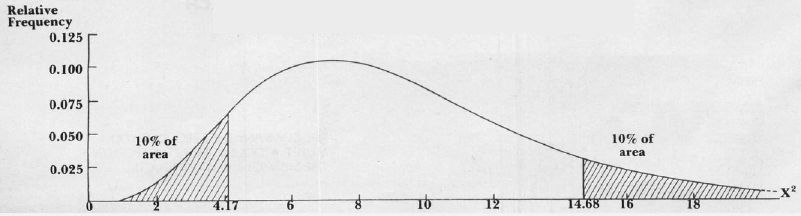
X2 = 12.07 for 100,000 executions of RND (0), grouped into 10 cells. As Figure 2 shows, 10% of all values in a chi-square distribution with nine degrees of freedom (number of cells minus one) are less than 4.2 and 10% are greater than 14.7. Our value does not fall within either of these extreme percentiles. The sequence of fractions cannot, therefore, be accused of non-randomness on the basis of this test alone.
One test, however, is not conclusive evidence of randomness. The X2 test performed on 100,000 numbers may suggest global randomness while hiding locally non-random behavior. For example, the distribution of the first 500,000 numbers generated by RND (0) may be skewed towards 0 while the distribution of the second 50,000 is skewed towards 1. The two distributions added together may appear uniform. To uncover such deception, the X2 test is performed on each successive block of 10,000 fractions, and on each cumulative block. Table 2 shows that the TRS-80 random number generator produces an acceptable X2 value in each case examined.
Batteries of statistical tests such as the chi-square will never prove that a random number generator is a good one, however. But they may diminish doubt, for each passed test boosts confidence in the quality of the generator. To strengthen or shatter this faith, sequences of TRS-80 fractions are now "RUNS" tested.
Let's explain this procedure using a list of Presidents of the United States and their political parties. We start with Franklin Pierce to avoid the Whigs and Federalists before him.
| PRESIDENT | PRESIDENT | ||
| Franklin Pierce | D | Woodrow Wilson | D |
| James Buchanan | D | Warren G. Harding | R |
| Abraham Lincoln | R | Calvin Coolidge | R |
| Andrew Johnson | R | Herbert Hoover | R |
| Ulysses S. Grant | R | Franklin D. Roosevelt | D |
| Rutherford B. Hayes | R | Harry S. Truman | D |
| James A. Garfield | R | Dwight D. Eisenhower | R |
| Chester Alan Arthur | R | John F. Kennedy | D |
| Grover Cleveland | D | Lyndon B.Johnson | D |
| Benjamin Harrison | R | Richard M. Nixon | R |
| Grover Cleveland | D | Gerald R. Ford | R |
| William McKinley | R | Jimmy Carter | D |
| Theodore Roosevelt | R | Ronald Reagan | R |
| William Howard Taft | R |
Are Democrats (D) and Republicans (R) randomly distributed here? Notice the string of six Republicans from Lindoln to Arthur. And notice that Grover Cleveland appears twice! Let's compare your guess to the probabilistic answer of the Runs Test. We first count the number of runs of Democrats or Republicans:
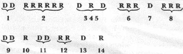
A run is a succession of identical symbols followed and preceded by the opposite symbol, or by no symbol at all. There are 14 runs in our sequence. The essence of the Runs Test is to determine if this number is "too many," or "too few," or "about right." "Too many" runs is best exemplified by a sequence where Democrats and Republicans perpetually alternate: D R D R D R … and so on. It is highly unlikely that a random sequence will follow a pattern so mechanical. "Too few" runs, on the other hand, is exemplified in its most grievous form by a sequence of all Democrats or all Republicans: R R R R R R … and so on. Again, it is highly unlikely that a random sequence will display this. The Runs Test formula (reference 2) is:
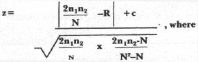
n1 = the number of Democrats
n2 = the number of Republicans
N = n1 + n2
R = the number of runs
This leaves "c," which is Yates' factor to make z's distribution better approximate a normal curve. Specifically,
c = +0.5 if R<2n1n2/N and c = -1.5 if R>2n1n2/N
Actually, the z-formula is supposed to be used only if n1 and/or n2 is more than 20; a special table is used otherwise. For our example, however, the table and the formula give the same result. We march with z to demonstrate its use.
In calculating z, first note that 2n1n2/N = 2*10*17/27 = 12.5926. With R = 14, c = -1.5.
Therefore:
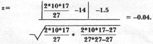
We reject with 95% confidence the assumption that a sequence is random whenever z = 1.96 or more. Since our calculated value is less than this, the Runs Test won't allow us to call the sequence of political parties non-random.
To "Runs" test a sequence of fractions, replace the "D's" and "R's" with "+'s" and "-'s." A "-" denotes a fraction below the expected median, 0.5, and a "+" denotes a fraction above it. For example, [.3 .7 .1 .2 .6] becomes [- + -- +]. Executing the Runs Test on 100,000 TRS-80 fractions, and on blocks therein, gives the results shown in Table 2. Each sequence appear random.
The computer program also generates four descriptive statistics useful in evaluating degree of randomness: mean and variance of the fractions, and covariance and correlation coefficient of successive fractions. The expected mean is 0.5, or the midpoint of the uniform distribution of Figure 1. The expected variance is 1/12; this can be derived using a bit of integral calculus. Finally, the remaining two statistics are expected to be zero since the elements of our sequence of numbers are supposed to be independent. Table 3 shows results for the first three statistics. All conform very closely to expectations.
The X2 test, the Runs Test, and a small battery of descriptive statistics suggest that RND (0) is a decent random number generator. But our evidence can never be conclusive, and the next test that we subject the generator to may be the one that it fails. So:
Be not too presumptuously sure in any business; for things of this world depend on such a train of unseen chances that if it were in man's hands to set the tables, still he would not be certain to win the game.
Herbert
References:
1. Knuth, Donald E. The Art of Computer Programming. Vol. 2. Reading: Addison-Wesley Publishing Company, 1971.
2. Langley, Russell. Practical Statistics Simply Explained. New York: Dover Publications, Inc., 1970.
| TABLE 1 Distribution Of The First 100,000 Fractions Generated By RND (0) | ||
| INTERVAL | TALLY | %OFTOTAL |
| 0.1 | 9969 | 9.97 |
| 0.1 to < 0.2 | 10084 | 10.08 |
| 0.2 to < 0.3 | 9980 | 9.98 |
| 0.3 to <0.4 | 9904 | 9.90 |
| 0.4 to <0.5 | 9985 | 9.99 |
| 0.5 to <0.6 | 10099 | 10.10 |
| 0.6 to <0.7 | 10098 | 10.10 |
| 0.7 to <0.8 | 9938 | 9.94 |
| 0.8 to <0.9 | 9774 | 9.77 |
| 0.9 | 10169 | 10.17 |
| Table 2. Test Results | ||||
| Cumulative Number Of Fractions Generated | X2 Values | "RUNS" Values | ||
| Block | Cumulative | Block | Cumulative | |
| 10,000 | 13.87 | 13.87 | 1.34 | 1.34 |
| 20,000 | 10.16 | 14.14 | 0.19 | 0.80 |
| 30,000 | 7.20 | 6.71 | 0.03 | 0.69 |
| 40,000 | 4.23 | 8.55 | 0.03 | 0.58 |
| 50,000 | 4.99 | 6.21 | 1.50 | 0.16 |
| 60,000 | 11.59 | 10.06 | 1.47 | 0.75 |
| 70,000 | 5.51 | 9.77 | 0.63 | 0.46 |
| 80,000 | 5.35 | 12.33 | 0.85 | 0.73 |
| 90,000 | 12.19 | 10.87 | 1.40 | 1.18 |
| 100,000 | 5.26 | 12.07 | 0.21 | 1.05 |
| Table 3. Descriptive Statistics | ||||||
| Cumulative Number of Fractions Generated | Mean Block Cumulative | Variance Block Cumulative | Covariance Block Cumulative | |||
| Expected Values | 0.500 | 0.083 | 0.000 | |||
| 10,000 | 0.498 | 0.498 | 0.085 | 0.085 | -0.001 | -0.001 |
| 20,000 | 0.499 | 0.499 | 0.083 | 0.084 | 0.001 | -0.000 |
| 30,000 | 0.499 | 0.499 | 0.083 | 0.084 | -0.001 | -0.000 |
| 40,000 | 0.499 | 0.499 | 0.083 | 0.083 | 0.001 | -0.000 |
| 50,000 | 0.502 | 0.500 | 0.083 | 0.083 | -0.000 | -0.000 |
| 60,000 | 0.503 | 0.500 | 0.083 | 0.083 | -0.000 | -0.000 |
| 70,000 | 0.504 | 0.501 | 0.084 | 0.083 | -0.001 | -0.000 |
| 80,000 | 0.501 | 0.501 | 0.084 | 0.084 | 0.001 | -0.000 |
| 90,000 | 0.496 | 0.500 | 0.084 | 0.084 | 0.001 | 0.000 |
| 100,000 | 0.501 | 0.500 | 0.083 | 0.083 | -0.000 | 0.000 |